Recommender Systems
Related Papers:
Making Recommendations
In a typical recommender system, you have some number of users as well as some number of items you want to recommend:
| Movie | Alice (1) | Bob (2) | Carol (3) | Dave (4) |
|---|---|---|---|---|
| Love at last | 5 | 5 | 0 | 0 |
| Romance forever | 5 | ? | ? | 0 |
| Cute puppies of love | ? | 4 | 0 | ? |
| Nonstop car chases | 0 | 0 | 5 | 4 |
| Swords vs. karate | 0 | 0 | 5 | ? |
- $n_u$ — number of users $(n_u=4)$
- $n_m$ — number of movies $(n_m=5)$
- $r(i,j)$ — 1 if user $j$ has rated movie $i$ $(r(3,1)=0)$
- $y^{(i,j)}$ — rating given by user $j$ to movie $i$; defined only if $r(i,j)=1$; $(y^{(3,2)}=4)$
With this framework for recommender systems, one possible way to approach the problem is to look at the movies that users have not rated and to try to predict how users would rate those movies, because then, we can try to recommend to users things that they are more likely to rate as five stars.
Collaborative Filtering
Collaborative filtering refers to an algorithm where we figure out appropriate features and therefore a rating for a particular movie based on collaborative ratings given by other users.
For a moment, let’s assume that we have features of each item (movie). In this case, we can use a linear regression approach with a weight and bias vectors + the feature vector of each movie to predict the rating for a movie per user.
| Movie | Alice (1) | Bob (2) | Carol (3) | Dave (4) | $x_1$ (romance) | $x_2$ (action) |
|---|---|---|---|---|---|---|
| Love at last | 5 | 5 | 0 | 0 | 0.9 | 0 |
| Romance forever | 5 | ? | ? | 0 | 1.0 | 0.01 |
| Cute puppies of love | ? | 4 | 0 | ? | 0.99 | 0 |
| Nonstop car chases | 0 | 0 | 5 | 4 | 0.1 | 1.0 |
| Swords vs. karate | 0 | 0 | 5 | ? | 0 | 0.9 |
- $n$ — number of features $(n=2)$
- $x^{(i)}$ — feature vector of movie $i$ ($x^{(1)}= \begin{bmatrix} 0.9 \ 0 \end{bmatrix}$)
- $(w^{(1)},b^{(1)})$ — parameters for user 1
- $m^{(j)}$ — number of movies rated by user $j$
For user 1: Predict rating for movie $i$ as: $w^{(1)} \cdot x^{(i)}+b^{(1)}$
For user $j$: Predict user $j$’s rating for movie $i$ as: $w^{(j)} \cdot x^{(i)}+b^{(j)}$
Cost Function
To learn $w^{(j)},b^{(j)}$ for user $j$:
\[min_{w^{(j)},b^{(j)}}J(w^{(j)},b^{(j)})=\frac{1}{2} \sum_{i:r(i,j)=1}(w^{(j)} \cdot x^{(i)} + b^{(j)} - y^{(i,j)})^2 + \frac{\lambda}{2}\sum_{k=1}^n (w_{k}^{(j)})^2\]To learn parameters $w^{(1)},b^{(2)}, w^{(2)},b^{(2)},\dots, w^{(n_u)},b^{(n_u)}$ for all users, minimize:
\[J \begin{pmatrix} w^{(1)}, \dots, w^{(n_u)} \\ b^{(1)}, \dots, b^{(n_u)} \end{pmatrix} = \frac{1}{2} \sum_{j=1}^{n_u} \; \sum_{i:r(i,j)=1}(w^{(j)} \cdot x^{(i)} + b^{(j)} - y^{(i,j)})^2 + \frac{\lambda}{2} \sum_{j=1}^{n_u} \; \sum_{k=1}^n (w_{k}^{(j)})^2\]Collaborative Filtering Algorithm
This time, let’s assume that we don’t have access to the feature vectors of the movies, but instead, we have ratings and the parameters $w,b$ for each movie. How do we learn the feature values to make predictions for movies?
| Movie | Alice (1) | Bob (2) | Carol (3) | Dave (4) | $x_1$ (romance) | $x_2$ (action) |
|---|---|---|---|---|---|---|
| Love at last | 5 | 5 | 0 | 0 | ? | ? |
| Romance forever | 5 | ? | ? | 0 | ? | ? |
| Cute puppies of love | ? | 4 | 0 | ? | ? | ? |
| Nonstop car chases | 0 | 0 | 5 | 4 | ? | ? |
| Swords vs. karate | 0 | 0 | 5 | ? | ? | ? |
Given $w^{(1)},b^{(2)}, w^{(2)},b^{(2)},\dots, w^{(n_u)},b^{(n_u)}$, to learn $x^{(i)}$, minimize:
\[J(x^{(i)})=\frac{1}{2} \sum_{j:r(i,j)=1}(w^{(j)} \cdot x^{(i)} + b^{(j)} - y^{(i,j)})^2 + \frac{\lambda}{2}\sum_{k=1}^n (x_{k}^{(i)})^2\]To learn $x^{(1)}, x^{(2)},\dots,x^{(n_m)}$, minimize:
\[J (x^{(1)}, x^{(2)},\dots x^{(n_m)})= \frac{1}{2} \sum_{i=1}^{n_m} \; \sum_{k:r(i,j)=1}(w^{(j)} \cdot x^{(i)} + b^{(j)} - y^{(i,j)})^2 + \frac{\lambda}{2} \sum_{i=1}^{n_m} \; \sum_{k=1}^n (x_{k}^{(i)})^2\]Notice that the main summation parts for both cost functions are the same. Therefore, to learn $w,b,x$, we can use the following cost function and regularize $w,b$ and $x$:
\[min \begin{pmatrix} w^{(1)}, \dots,w^{(n_u)} \\ b^{(1)}, \dots, b^{(n_u)} \\ x^{(1)}, \dots, x^{(n_m)} \end{pmatrix} J (w,b,x)= \frac{1}{2} \sum_{(i,j):r(i,j)=1}(w^{(j)} \cdot x^{(i)} + b^{(j)} - y^{(i,j)})^2 + \frac{\lambda}{2} \sum_{j=1}^{n_u} \; \sum_{k=1}^n (w_{k}^{(j)})^2 + \frac{\lambda}{2} \sum_{i=1}^{n_m} \; \sum_{k=1}^n (x_{k}^{(i)})^2\]Gradient Descent
Using this knowledge, to minimize $w,b,x$, we can apply the following gradient descent algorithm to get to a set of good values for those parameters.
Repeat until convergence:
\[\begin{align*} w_{i}^{(j)} &\leftarrow w_{i}^{(j)} - \alpha \frac{\partial}{\partial w_{i}^{(j)}} J(w,b,x) \\ b^{(j)} &\leftarrow b^{(j)} - \alpha \frac{\partial}{\partial b^{(j)}} J(w,b,x) \\ x_{k}^{(i)} &\leftarrow x_{k}^{(i)} - \alpha \frac{\partial}{\partial x_{k}^{(i)}} J(w,b,x) \end{align*}\]Binary Labels - From Regression to Binary Classification
When the data we’re working with comes in binary levels (likes, dislikes, etc.), the Collaborative Filtering algorithm changes a little bit.
Example applications:
- Did user $j$ purchase an item after being shown? (yes=1, no=0, not_shown=?)
- Did user $j$ fav/like an item?
- Did user $j$ spend at least 30 seconds with an item?
- Did user $j$ click on an item?
Meaning of ratings?
1 - engaged after being shown an item
0 - did not engage after being shown an item
? - item not yet shown
Previously:
- Predict $y^{(i,j)}=w^{(j)} \cdot x^{(i)}+b^{(j)}$
For Binary Labels:
- Predict that the probability of $y^{(i,j)}=1$ is given by $g(w^{(j)} \cdot x^{(i)}+b^{(j)})$ where $g(z)=\frac{1}{1+e^{-z}}$
Cost Function
\[y^{(i,j)}= g(w^{(j)} \cdot x^{(i)}+b^{(j)}) \newline\] \[L(f_{(w,b,x)}(x),y^{(i,j)}= -y^{(i,j)}log(f_{(w,b,x)}(x))-(1-y^{(i,j)})log((1-f_{(w,b,x)}(x))\] \[J(w,b,x)=\sum_{(i,j):r(i,j)}L(f_{(w,b,x)}(x),y^{(i,j)})\]Mean Normalization
Mean normalization can help the algorithm run more efficiently.
For instance, if there is a person with no ratings available, mean normalization will help the algorithm make better predictions for that individual. Otherwise, the regularization term for $w$ will drive it down to $0$ since there are no ratings available and gradient descent tries to minimize it.
To apply mean normalization, compute a vector consisting of each movie’s mean (average of each row), and subtract the vector from the (movies X users) matrix.
Then, for user $j$ on movie $i$ predict: $w^{(j)}\cdot x^{(i)}+b^{(j)}+\mu_i$
This way, a person with no ratings with get a prediction of $\mu_i$
TensorFlow Implementation
To implement Collaborative Filtering, let’s first see how Auto Diff works, so we can utilize it to automatically compute the gradient of the cost function:
w = tf.Variable(3.0) # tells TF it's a parameter we want to optimize
x = 1.0
y = 1.0 # target value
alpha = 0.01

iterations = 30
for iter in range(iterations):
	# Use TF's Gradient tape to recrod the steps
	# used to compute the cost J to enable auto differentiation.
	# Auto Diff / Auto Grad
	with tf.GradientTape() as tape:
		# assuming the cost function is J=(wx-1)^2
		fwb = w*x
		costJ = (fwb - y)**2

	# Use the gradient tape to calculate the gradients
	# of the cost with respect to the parameter w.
	[dJdw] = tape.gradient(costJ, [w])

	# Run one step of gradient descent by updating
	# the value of w to reduce the cost.
	w.assign_add(-alpha * dJdw)
Using this knowledge, let’s now see the full implementation:
# instantiate an optimizer
optimizer = keras.optimizers.Adam(learning_rate=1e-1)

iterations = 200
for iter in range(iterations):
	# Use TF's Gradient Tape
	# to record the operations used to compute the cost
	with tf.GradientTape() as tape:

		# compute the cost (forward pass is included in cost)
		cost_value = costFunctionV(X, W, b, Ynorm, R,
			num_users, num_movies, lambda)

	# Use the gradient tape to automatically retrieve the
	# gradients of the trainable variables with respect to the loss
	grads = taoe.gradient(cost_value, [X,W,b])

	# Run one step of gradient descent by updating
	# the value of the variables to minimize the loss
	optimizer.apply_gradient(zip(grads, [X,W,b]))
Finding Related Items
The features $x^{(i)}$ of item $i$ are quite hard to interpret.
To find other items related to it, find item $k$ with $x^{(k)}$ similar to $x^{(i)}$, i.e. with smallest distance:
\[||x^{(k)}-x^{(i)}||=\sum_{l=1}^{n}(x^{(k)}_l - x^{(i)}_l)^2\]Limitations of Collaborative Filtering
Cold start problem — how to:
- rank new items that few users have rated?
- show something reasonable to users who have rated few items?
Doesn’t give us a natural way to use side information about items or users:
- Item: Genre, movie stars, studio, …
- User: Demographics (age, gender, location), expressed preferences, …
Content-Based Filtering Algorithm
Collaborative filtering: Recommend items to you based on ratings of users who gave similar ratings as you
Content-based filtering: Recommend items to you based on features of the user and the item to find good match
User features $(x_{u}^{(j)}$ for user $j)$
- Age
- Gender (1 hot)
- Country (1 hot - 200)
- Movies watched (1 hot — 1000 pop. movies)
- Average rating per genre
Movie features $(x_{i}^{(m)}$ for movie $i)$
- Year
- Genre/Genres
- Reviews
- Average rating
- $\dots$
Given these features, we want to figure out whether movie $i$ is going to be a good match for user $j$.
Also, notice that the features for users and movies may not match in size, and that’s okay.
Learning to Match
Predict rating of user $j$ on movie $i$ as: $v_{u}^{(j)} \cdot v_{m}^{(i)}$
- $v_{u}^{(j)}$ — computed from $x_{u}^{(j)}$
- $v_{m}^{(i)}$ — computed from $x_{m}^{(i)}$
Although the dimensions of the feature vectors may not match for users and movies, their respective vectors $v$ should match in size.
To compute these vectors, we’ll use Deep Learning.
Deep Learning for Content-Based Filtering
Below is a possible architecture for computing the vectors for movies and users given their features/preferences:
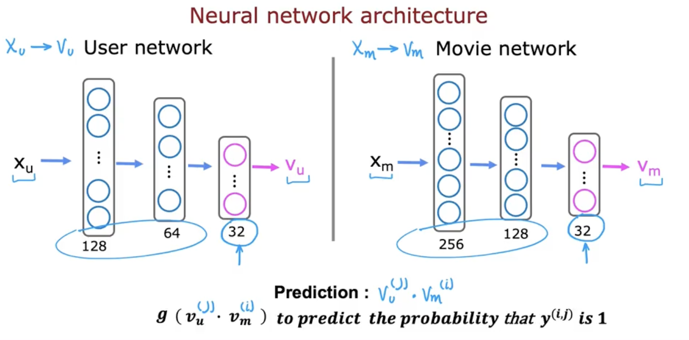
To judge the performance of the neural nets, we use the following cost function:
\[J= \sum_{(i,j):r(i,j)=1} (v_{u}^{(j)}\cdot v_{m}^{(i)} - y^{(i,j)})^2 + NN\; reg.\; term\]We can also utilize this function to find similar functions like we did with collaborative filtering.
Finding Related Items
$v_{u}^{(j)}$ — a vector of length 32 that describes user $j$ with features $x_{u}^{(j)}$
$v_{m}^{(i)}$ — a vector of length 32 that describes user $i$ with features $x_{m}^{(i)}$
To find movies similar to $i$, find a movie $k$ that results in small:
\[||v_{m}^{(k)}-v_{m}^{(i)}||^2\]Note: This can be pre-computed
Recommending from a Large Catalogue
Oftentimes, you will have the following scenario:
- Movies — 1000+
- Ads — 1m+
- Songs — 10m+
- Products — 10m+
So, running a neural network inference millions of times for all the items is computationally infeasible.
To aid this, we can use the two step process: Retrieval & Ranking
Retrieval:
- Generate a large list of plausible item candidates:
- For each of the last 10 movies watched by the user, find 10 most similar movies (^finding related items)
- For most viewed 3 genres, find the top 10 movies
- Top 20 movies in the country
- Combine retrieved items into a list, removing duplicates and items already watched/purchased, ending in probably 100s of movies.
Ranking:
- Take the retrieved list and rank the movies passing it (and the user vector) through the neural network and take the dot product.
- Display the ranked items to the user
- If you have computed $v_m$ for all the movies in advance, all you have to do is compute $v_u$ and take the dot product, making inference really fast.
TensorFlow Implementation
user_NN = tf.keras.models.Sequential([
	tf.keras.layers.Dense(256, activation='relu'),
	tf.keras.layers.Dense(128, activation='relu'),
	tf.keras.layers.Dense(32)
])

item_NN = tf.keras.models.Sequential([
	tf.keras.layers.Dense(256, activation='relu'),
	tf.keras.layers.Dense(128, activation='relu'),
	tf.keras.layers.Dense(32)
])

# create the user input and point to the base network
input_user = tf.keras.layers.Input(shape=(num_user_features))
vu = user_NN(input_user)
vu = tf.linalg.l2_normalize(vu, axis=1) # makes the alg work better ??

# create the item input and point to the base network
input_item = tf.keras.layers.Input(shape=(num_item_features))
vm = item_NN(input_item)
vm = tf.linalg.l2_normalize(vm, axis=1)

# measure the similarity of the two vector outputs
output = tf.keras.layers.Dot(axes=1) ([vu, vm])

# specify the inputs and output of the mdoel
model = Model([input_user, input_item], output)

# specify the cost function
cost_fn = tf.keras.losses.MeanSquaredError()