• Why Feature Selection?
• Structure
• Levels of Measurement
• Filter Methods
  • Pearson’s R
  • Kendall’s Tau
  • Spearman’s Rho
  • Chi-Squared $(\chi^2)$ Test
  • Mutual Information
  • ANOVA F-Score
  • Point-Biserial $(r_{pb})$
• Summary
• Appendix

Why Feature Selection?

Let’s say that you’re a junior Machine Learning Engineer working at a bank, and you’ve been tasked with building a model that predicts if a customer will default on a loan or not. Before you build your classifier, you talk to your colleagues in Analytics, and they claim that there are approximately 500 factors that go into determining if someone is unable to pay their loans. You, however, want to find top 15 most relevant features to train your classifier with because you want to keep your model light and transparent. How do you proceed? In other words, how do you go from 500 features overall down to just 15 best?

Whether you want to simplify your model, reduce training time, address the above scenario, or follow any one of these uses of Feature Selection, you will want to learn a few good methods to select top $k$ features before you start training your model.

That’s what I hope you’ll take away from this article. I know there are hundreds (if not thousands) of guides on this very topic on the internet, but very few of them focus on the statistical background of these methods. I noticed that they all just talk about Feature Selection on a surface level instead of digging deep into the theory and hard math involved in the process, which I think is essential if you want to build strong intuition around Feature Selection methods and master them well.

Structure

This article will be structured in the following way: first, I’ll walk you through a short introduction to a method; second, I’ll cover any prerequisites that you will probably need to understand the method — for example, explaining what Covariance is before the Correlation Coefficient. Then, I’ll go over the formula plus the math behind how the method works (if there is any) to build intuition for how/why the method works, and also for when this method is applicable. Finally, I’ll tie everything up and provide an implementation in code to make sure you’ve fully grasped the concept and are ready to apply it for your own case.

Note that some mathematical concepts mentioned throughout the article (expectation, variance, etc.) are re-occurring, so to avoid explaining them every time they’re mentioned, I’ve put them in the Appendix. If you’re unfamiliar with these concepts, I strongly suggest that you spend a bit of time understanding them, as they’re a crucial part of every major feature selection method.

For the record, there are many approaches to feature selection, and all of them are usually grouped into four families of methods: Unsupervised and Supervised, which in itself consists of three groups: Wrapper methods, Filter methods, and Embedded methods. In this blog, we’ll discuss the most commonly used family of methods — Filter. Filter methods rely on analyzing each feature’s statistical relationship with the target variable as an indicator for the model’s performance. They’re fast, easy, and quite convenient to work with if you’re tackling classical ML problems.

If you want to read more about the other families of feature selection methods, here’s a link to Wrapper methods, and this is a Wikipedia reference to all the methods.

Levels of Measurement

Alright, one last thing before we start discussing Filter methods, I promise. We first have to agree on what “kind” of data we are looking at while doing feature selection. What I mean is, in statistics, data isn’t just numbers or text; it falls into a specific hierarchy of information known as the Levels of Measurement, so I’ll try explaining it here the way I was taught in college.

There are four levels of measurement, ranging from the simplest (least information) to the most complex (most information):

1. Nominal: This is data that acts only as a label; i.e. there is no order and no distance.
   • Examples: $Eye Color (Blue, Brown, …), City (Tashkent, Ithaca, …).$
   • You can only count them; for instance, you can’t say $”Blue > Brown”$.
2. Ordinal: This is data where the order matters, but the distance between values is unknown or inconsistent.
   • Examples: T-Shirt Sizes $(S, M, L)$, Satisfaction Surveys $(Good, Neutral, Dogsh*t).$
   • You can say $”L > M”$, but you can’t say “$L-M=S$.”$\;$ In other words, you know the direction, but you don’t know the scale of difference.
3. Interval: Here, the order matters and the distance between values is equal and meaningful. However, there is no “True Zero” (a zero point doesn’t mean “none” or “absence”).
   • Examples: Temperature in Celsius/Fahrenheit ($0^\circ C$ is cold, not “no heat”), Calendar Years (Year 0 isn’t the beginning of time).
   • You can add and subtract, but you cannot multiply or divide. You can’t say “$20^\circ C$ is twice as hot as $10^\circ C$” (yeah, this kind of took me by surprise when I first learned about it too).
4. Ratio: This is the highest level of data. It has order, equal distance, and a “True Zero” (0 means the total absence of the variable).
   • Examples: Height, Weight, Salary, Counts (0 items sold), Age, etc.
   • You can do everything. Because zero is real, you can say “A person weighing 100 kilos is exactly twice as heavy as someone weighing 50”.

The reason I’m talking about Levels of Measurement in data is that feature selection methods are strict about this hierarchy. What I mean is, you cannot use a method designed for Ratio data (like Pearson’s $r$) on Nominal data. However, you generally can use a method designed for a lower levels (like Nominal) on higher levels (like Ratio) by kind of “downgrading” your data; for example, grouping you friends’ ages into age buckets.

Cool? Alright, let’s get started.

Filter Methods

Pearson’s R:

The first filter method we’re going to look at is Pearson’s $r$ (correlation coefficient). The correlation coefficient measures the strength and the direction of a linear relationship between two variables, and it does so by measuring the Covariance between them.

For two variables $X$ (age of every student in a classroom) and $Y$ (height of every student in a classroom), with respective means $\mu_X$ and $\mu_Y$, the covariance between $X$ and $Y$ is defined as

Let me explain what this formula computes:

• $(X-\mu_X)$: each student’s age minus the average age in the classroom
• $(Y-\mu_Y)$: each student’s height minus the average height in the classroom
• $P=(X-\mu_X)(Y-\mu_Y)$: let’s temporarily define this as the product of the two differences
• $E[P]$: this measures the expected value of $P$. In other words, it measures the weighted average of the values of $P$ (if this is unclear, see the appendix on Expectation). You can interpret this as the average product between $[$the differences for each student’s age, height and their corresponding averages$]$.

Covariance will be positive when large values of $X$ are associated with large values of $Y$ and small values of $X$ are associated with small values of $Y$. On the other hand, if $X$ are $Y$ are inversely related, most product terms will be negative, as when $X$ takes values above the mean, $Y$ will tend to fall below the mean, and vice versa.

Covariance is a measure of linear association between two variables. In a sense, the “less linear” the relationship, the closer the covariance is to 0.

The sign of the covariance indicates whether two random variables are positively or negatively associated. But the magnitude of the covariance can be difficult to interpret due to the scales of the original variables, which is where the correlation coefficient comes in.

Pearson’s $r$, takes the covariance between two variables and divides it by the product of their respective standard deviations - a measure of variation around the mean (see the appendix on what that is), thus making the correlation fall in the range of $[-1,1]$ and the value meaningful.

The properties of correlation are as follows:

1. $-1 \leq Corr(X,Y) \leq 1$
2. If $Y=aX+b$ is a linear function of $X$ for constants $a$ and $b$, then $Corr(X,Y)= \pm1$, depending on the sign of $a$.

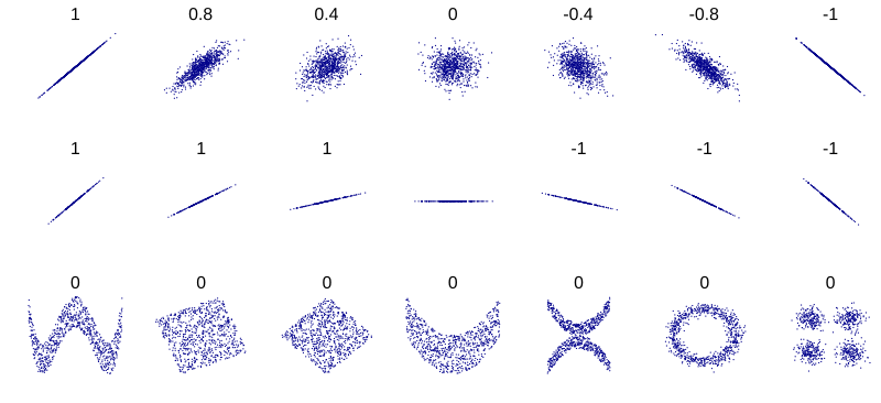
The first property says the correlation coefficient is always between $-1$ and $1$ (see this section if you’re interested in a proof). If it is $-1$ or is close to it, that means there is a strong negative linear association between the two variables; if it’s around $1$, the relationship is still strong but positive. As the coefficient approaches $0$, the association between the variables also diminishes.

The second property states that when the correlation coefficient of two variables $X$ and $Y$ is exactly $1$ or $-1$, then we can express one variable as a perfect linear function of the other with no random noise whatsoever, meaning the two variables are perfectly correlated.

Pearson’s R is applicable when the features are of the following categories:

• $X$: interval/ratio
• $Y$: interval/ratio

While selecting the “best” features for our model, the higher the Correlation Coefficient between a feature and our target variable, the better. If you wanted to build a model that predicts the Height of a student based on a number of factors, including their Age and the Number of siblings they have, you might find that Pearson’s $r$ between Height and Age is pretty high while the coefficient between Height and Number of siblings is pretty low. In this case, you should keep the first feature.

Code:

from scipy.stats import pearsonr

# x and y are continuous
corr, p_value = pearsonr(x, y)

print(f"Pearson Correlation: {corr:.3f}")
print(f"P-value: {p_value:.3e}")

Kendall’s $\tau$:

Relevant:

• https://en.wikipedia.org/wiki/Rank_correlation
• https://en.wikipedia.org/wiki/Kendall_rank_correlation_coefficient

The next method in our toolkit is Kendall’s Tau, which is also known as Kendall’s rank correlation coefficient. Hopefully, from the previous section you know that Pearson’s $r$ measures the strength and direction of a linear relationship; Kendall’s $\tau$ on the other hand, measures the strength of an Ordinal **association between two variables.

To give an example, it answers the question “When variable $X$ gets bigger, does variable $Y$ also tend to get bigger (or smaller for that matter)?”. It doesn’t care how much bigger, only that the direction of the relationship is consistent.

Again, before we go into any formulas, I think it’s crucial to understand the building blocks of Kendall’s $\tau$, which are its concordant and discordant pairs. In order to calculate the coefficient $\tau$, we look at every possible pair of observations in our dataset (if you’re familiar with combinatorics, you’ll know that for $n$ observations, you’ll have to consider $\binom{n}{2}=\frac{n!}{2!(n-2)!}$ pairs!). For any two observations $i$ and $j$, we have the values $(x_i,y_i)$ and $(x_j,y_j)$ — the corresponding values of variables $x$ and $y$ for observations $i$ and $j$.

1. Concordant Pair: A pair is concordant if the ranks of both variables move in the same direction, and this pair is expressed as $N_c$. This means that either $(x_i>x_j$ and $y_i>y_j)$, OR $(x_i<x_j$ and $y_i<y_j)$
2. Discordant Pair: A pair is discordant if the ranks of the variables move in opposite directions. This pair is expressed as $N_d$. This means either $(x_i>x_j$ and $y_i<y_j)$ , OR $(x_i<x_j$ and $y_i>y_j)$
3. Tied Pair: if $x_i=x_j$ or $y_i=y_j$ (we’ll come back to this).

Let’s put this all into practice with an example. Imagine we are ranking employees based on their Years of Experience and Bug Fixing Rank, where 1 is the best rank.

There are $n=3$ employees, so the total number of pairs is $\binom{3}{2}=\frac{3!}{2!(3-2)!}=3$. Let’s look at each pair:

1. (Linus, Steve)
   • Experience: $2<5$; $X$ increased.
   • Rank: $3>1$; $Y$ decreased (although a rank of 1 IS better than 3, the number 1 is still less than 3)

   So this is a discordant pair.

2. (Linus, Lola)
   • Experience: $2<3$; $X$ increased
   • Rank: $3>2$; $Y$ decreased

   This is also a discordant pair

3. (Steve, Lola)
   • Experience: $5>3$; $X$ decreased
   • Rank: $1<2$; $Y$ increased

   This is also a discordant pair

Alright, in this example, we have 0 concordant pairs and 3 discordant pairs. Intuitively, this shows a perfect negative relationship: as experience goes up, the rank number goes down (i.e. the productivity rank gets better).

Kendall’s $\tau$ is essentially the difference between the number of concordant and discordant pairs, normalized to fall between -1 and 1. Tau-a:

The simplest version of the Tau statistic is Tau-a, or $\tau_A$ and is used when there are no ties in the data, as in no two $x$ values are the same and no two $y$ values are the same. The formula for it is:

For our example above,

This shows a perfect negative ordinal relationship, just as we had predicted.

Tau-b:

In the real world though…., data almost always have ties. What if Linus and Steve both had 2 years of experience? Then the (Linus, Steve) pair would tied on X (Years of Experience).

The formula for $\tau_A$’s denominator becomes inaccurate because it assumes all pairs are either concordant or discordant (i.e. the denominator overcounts because some pairs can’t be classified as concordant or discordant at all), so we need a way to handle these ties. This is where $\tau_B$ comes in. It’s the most common version of Kendall’s correlation, and the formula adjusts the denominator to account for pairs that are tied on $x$ $(T_x)$ and pairs that are tied on $y$ $(T_y)$. The numerator is the same, but the denominator becomes the geometric mean (Appendix D) of the total pairs excluding ties on $x$ and the total pairs excluding ties on $y$.

The properties of Kendall’s $\tau$ are as follows:

• $-1\leq\tau \leq1$
• $\tau=1$: Perfect agreement. All pairs are concordant. If you sort the data by variable $x$, variable $y$ will also be perfectly sorted in ascending order.
• $\tau=-1$: Perfect disagreement. All pairs are discordant. If you sort the data by variable $x$, variable $y$ will be perfectly sorted in descending order.
• $r=0$: No association. The number of concordant and discordant pairs is equal. The variables are independent.

A key advantage of Kendall’s $\tau$ over Pearson’s $r$ is that it can capture non-linear monotonic relationships. Pearson’s $r$ only measures linearity.

For example, let’s consider a case where as $x$ increases, $y$ always increases, but not in a straight line. Pearson’s $r$ would be positive, but not 1, Kendall’s $\tau$, on the other hand, (and Spearman’s, which we’ll see soon) would be exactly 1 because every single pair of points is concordant.

Kendall’s $\tau$ is applicable when the features are of the following categories:

• $X$: ordinal, interval, ratio

• $Y$: ordinal, interval, ratio

  Ordinal, because this is its native territory. Data like small, medium, large or good, neutral, bad can be directly compared to form concordant/discordant pairs.

  Interval/ratio, because data like temperature or salary have a natural order, so they can easily be converted into buckets of ranks

  As you already might have guessed, you can’t use $\tau$ with data like car, boat, plane, etc. because there is no logical order to them, that is you can’t say car > boat. It’s impossible to form a concordant or discordant pair.

Code:

from scipy.stats import kendalltau

# x and y can be ordinal or continuous
tau, p_value = kendalltau(x, y)

print(f"Kendall’s Tau: {tau:.3f}")
print(f"P-value: {p_value:.3e}")

Spearman’s $\rho$:

Relevant:

• https://en.wikipedia.org/wiki/Spearman’s_rank_correlation_coefficient

Now, let’s talk about Spearman’s rank correlation coefficient, also known as Spearman’s Rho. This method is a very close cousin (brother even) to both Pearson’s $r$ and Kendall’s $\tau$ — here’s a link the Wikipedia page if you’re curious about that.

• Like Kendall’s $\tau$, it measures the strength and direction of a monotonic relationship
• Like Pearson’s $r$, it’s calculated using a familiar formula, but with a clever twist

Essentially, Spearman’s $\rho$ answers the question ‘How well can the relationship between two variables be described by a monotonic function?’. In other words, as one variable increases, does the other consistently increase or decrease, even if not at a constant rate?

The ‘twist’ behind Spearman’s $\rho$ I mentioned earlier is very elegant and easy to understand (if you understood Pearson’s $r$ that is):

Spearman’s $\rho$ is simply Pearson’s $r$ calculated on the ranks of the data, not on the data itself. That’s it!!

Instead of using raw values like $X=3,7,11$, you first convert them to ranks $X_{rank}=1,2,3$ and then use the Pearson’s $r$ formula on those ranks.

Let’s formalize this:

1. Take your two variables $X$ and $Y$
2. For variable $X$, rank all its observations from smallest to largest. The smallest value gets rank 1, next smallest gets rank 2, and so on. Let’s call this new function $rank(X)$
3. Do the exact same thing on $Y$. Let’s also call this $rank(Y)$
4. Now calculate Pearson’s $r$ between $rank(X)$ and $rank(Y)$:

By converting the raw values to ranks, you’ve thrown away all information about magnitude and distribution. You are left with only the order. This is what allows Spearman’s to detect a perfect monotonic relationship even if it’s not linear.

The properties of Spearman’s $\rho$ are as follows:

• $-1\leq\rho\leq1$
• $\rho=1$: Perfect positive monotonic relationship. As $X$ increases, $Y$ never decreases.
• $\rho=-1$: Perfect negative monotonic relationship. As $X$ increases, $Y$ never increases.
• $\rho=0$: No monotonic relationship

Alright, let’s get our hands dirty and go through a non-linear example:

A Pearson’s $r$ calculation on $X$ and $Y$ would not be 1 here. It would be high, but not 1 because the relationship is not a straight line because $Y$ isn’t a linear function of $X$.

A Spearman’s $\rho$ calculation would first find the ranks:

• $rank(X)=[1,2,3,4,5]$
• $rank(Y)=[1,2,3,4,5]$

And since $rank(X)$ and $rank(Y)$ are identical, the correlation between them is a perfect 1.

Spearman’s $\rho$ correctly shows this as a perfect relationship, whereas Pearson’s $r$ does not. This also shows that $\rho$ is less sensitive to outliers than $r$ — an outlier might drastically change the mean and SD (affecting $r$), but it will only change its rank by one position, having a minimal effect on $\rho$. Cool, right?

You might be asking yourself right now if Spearman and Kendall are the same. In a way, they are: they both measure monotonic relationships, so for feature selection, they will almost always lead you to the same conclusions in the same setting. So, it’s really up to you to decide which one to use, this stack exchange post discusses this very question.

Because Spearman’s $\rho$ is based entirely on ranks, its applicability is identical to Kendall’s $\tau$:

• $X$: ordinal, interval, ratio
• $Y$: ordinal, interval, ratio

See the same section in Kendall’s $\tau$ to see why.

Code:

from scipy.stats import spearmanr

# x and y can be ordinal and continuous
rho, p_value = spearmanr(x, y)

print(f"Spearman’s Rho: {rho:.3f}")
print(f"P-value: {p_value:.3e}")

Chi-Squared $(\chi^2)$ Test:

Alright, it gets interesting now. The methods we’ve discussed so far are designed to measure the correlation between variables that have some kind of order to them (ordinal, interval, or ratio). BUT, what if our variables are purely categorical, like ‘City’ $(X)$ or ‘Clicked Post’ $(Y)$? Obviously there is no natural order to ‘Berlin’, ‘Bukhara’ and ‘Bern’, so we can’t rank them or calculate a correlation. If, for some reason, you wanted to use the city someone lives in as a feature in your ML model, how exactly would you do so?

As you might’ve guessed, this is where the $\chi^2$ test comes in: Instead of measuring the correlation, the $\chi^2$ test measures independence. In other words, it answers the question “Are these two categorical variables independent of each other?”.

For feature selection, we want the opposite. We want features that are dependent on our target variable. If a feature is dependent on the target, it means knowing the feature’s value gives us information about the target’s value, so you’d better have it in your model.

The entire $\chi^2$ test is built on comparing the data we see with the data we would expect to see if the two variables were perfectly independent (in the statistical world this is called Observed vs Expected).

The first step in doing this is to put our data in a Contingency Table, which is the default way to summarize two categorical variables in statistics. Let’s do that and use an example where we measure the amount of times 1000 people played three video games.

Now, we must calculate the Expected Frequencies $EF$ (this is the most important concept in this section). The expected frequency for a cell is the count we would see if the variables were totally independent from each other. The way we calculate the expected frequencies is as follows:

For Factorio, “Played: Yes”:

1. Overall, what’s the probability of someone playing a game? Well, it’s $130/1000=13\%$
2. Overall, how many people play Factorio? $500$
3. If the play rate is independent of the game, then we would expect the $13\%$ play rate to apply to Factorio fans just like everyone else.
4. Therefore, $EF(game, Yes)=13\%$ of $500=0.13\times500=65$. This number says that if the fact that whether someone plays a game or not is independent from the kind of the said game, we’d expect 65 people to play Factorio.

The general formula for any cell’s expected frequency is:

Plugging in the numbers from the above example, we get: $\frac{500\times130}{1000}=65$; same as before!

Using the formula, let’s build the expected frequencies table for all the games:

Now, we look at the two tables:

• Observed (Factorio, Yes): $90$
• Expected (Factorio, Yes): $65$

As you can see, that’s a big difference! This discrepancy is the evidence that our variables might not be independent.

The $\chi^2$ Statistic: The Formula

The formula for computing the $\chi^2$ statistic uses the logic above, and the output is simply a single number that shows the total difference between the Observed $(O)$ and Expected $(E)$ tables. We calculate the difference for each cell, and then sum them all up.

The formula is:

Let’s break this down:

1. $(O-E)$: The difference for one cell. (e.g., $90-65=25)$
2. $(O-E)^2$: We square difference. This does two things: First, it makes all differences$\;$ positive, so they don’t cancel each other out. Second, it heavily penalizes large differences.
3. $\frac{\dots}{E}$: We normalize$\;$the difference by dividing by the expected value. This is crucial. A difference of $10$ is massive if you only expected $5$, but it’s trivial if you expected $10,000$. So this puts all differences on a relative scale.

Let’s calculate it for our example (summing $\frac{(O-E)^2}{E}$ for all $6$ sells):

• (Factorio, Yes): $\frac{(90-65)^2}{65} = 9.62$
• (Factorio, No): $\frac{(410-435)^2}{435}=1.44$
• (Devil Daggers, Yes): $\frac{(30-39)^2}{39}=2.08$
• (Devil Daggers, No): $\frac{(270-261)^2}{261}=0.31$
• (Icy Tower, Yes): $\frac{(10-26)^2}{26}=9.85$
• (Icy Tower, No): $\frac{(190-174)^2}{174}=1.47$

So, the total $\chi^2$ value is: $\chi^2=9.26+1.44+2.08+0.31+9.85+1.47=24.77$

Interpretation and Properties:

• Range: The $\chi^2$ value is always $\ge 0$. It can never be negative, because all the terms are squared.
• $\chi^2=0$: This would mean that $O=E$ for every single cell. The observed data perfectly matches the ‘independent’ model. This is the worst possible score for feature selection, as it means the feature is $100\%$ independent of the target.
• $\chi^2 > 0$: The larger the $\chi^2$ value, the greater the discrepancy between your observed data and the ‘independent’ model.
• For Feature Selection: We rank our features by their $\chi^2$ score. A higher $\chi^2$ score means the ‘null hypothesis’ (that they are independent) is less likely. This suggests a stronger association/dependency between the feature and target, which makes it a better feature.

In our example, $\chi^2=24.77$ is significantly high, telling us that ‘Video Game’ is almost certainly not independent of ‘Played Game’ and is therefore a good feature to keep.

Variable Applicability:

This is the most important part. The Chi-Squared test operates on counts within discrete categories, so it is applicable when the features are of the following categories:

• $X$: Nominal, Ordinal
• $Y$: Nominal, Ordinal

Nominal, because this is its primary use case. ‘Type’, ‘Country’, ‘Color’, etc. are perfect. Ordinal, because it works perfectly for ordinal data (’Low’, ‘Medium’, ‘High’) as well, because it just treats them as distinct categories. However, it ignores the order information.

You cannot run a $\chi^2$ test on raw continuous variables like ‘Age’ or ‘Price’ because there are no discrete categories to build a contingency table with. Except:, there is a workaround: binning. To use $\chi^2$ with a continuous variable you can first bin it to convert it into an ordinal variable. For example, you could bin ‘Age’ into [’18-30’, ‘31-50’, ‘51+’]. The test is then run on these new bins, not the original data.

Code:

from sklearn.feature_selection import chi2, SelectKBest

# x is a categorical feature in the form of integers
# y is a categorical target
scores, p_values = chi2(X, y)

# you can automatically pick top 5 features
selector = SelectKBest(score_func=chi2, k=5)
X_new = selector.fit_transform(X, y)

Mutual Information (MI)

I hope you’re having fun. If not, you definitely will in this section.

So, we’ve looked at Pearson (linear relationships), Spearman/Kendall (monotonic relationships), and Chi-Squared (independence).

Let me ask you this: what happens when the relationship is weird? For example, what if the relationship is a sine wave? A circle? What if the relationship is “The target is 1 only when $X$ is between $5$ and $10$, otherwise it’s $0$”?

Linear and rank-based approaches will fail here. They might say the correlation is $0$, but the variables are obviously related - just not in a simple straight line.

This is where Mutual Information comes in. MI is a generalist approach to feature selection; it detects any kind of relationship between a feature and a target whether it be linear, non-linear, monotonic, or something really complex. To understand MI and how it works, we first need to go over the concept of Entropy which is a measure of uncertainty.

• Hight Entropy: you have no idea what’s going to happen (you toss a fair coin, and it could be heads or tails with 50/50 probability)
• Low Entropy: you’re pretty sure what’s going to happen (a biased coin that lands on heads with a 90% probability)
• Zero Entropy: you know exactly what will happen (a fraudulent coin with heads on both sides).

Mathematically, the entropy of a variable $Y$ is defined as:

If the formula doesn’t make sense to you, think of the log term as a measure of surprise. For example, if an event is guaranteed $(p=1)$, then $\log(1)=0$. In other words, there is zero surprise, so zero entropy. On the other hand, if an event is rare $(p=0.01)$, the the log value is large — it is surprising.

The formula calculates the weighted average of surprise. We multiple the surprise of an event $\log(p(y))$ by how often that even actually happens $(p(y))$.

Mutual Information answers a simple question: “How much does knowing variable $X$ reduce the uncertainty about variable $Y$?”

Imagine $Y$ is “Will it rain tomorrow?”

Scenario A: I tell you $X=$ “the result of a coin toss I just did”. Does knowing the coin toss result reduce your uncertainty about the rain? I hope not. Therefore, the Mutual Information is 0.

Scenario B: I tell you $X=$ “the humidity level right now”. Does knowing the humidity reduce your uncertainty about the rain? Yes. If humidity is high, you’re more sure it will rain. The Mutual Information is high in this case.

In essence, MI is the intersection of information between two variables. It is the information they share.

Now, let’s move on to the formula. The formula for MI is the total uncertainty of $Y$ minus the uncertainty that remains after knowing $X$. Pretty intuitive, right?

Let’s dissect this:

1. $H(Y)$ — the initial entropy of your target; in other words, “how hard is it to guess $Y$ without any clues?”.

2. $H(Y|X)$ — the conditional entropy; in other words, “how hard is it to guess $Y$ after I’ve given you the clue $X$?”.

It should now be easy to conclude that if $X$ is a perfect predictor, $H(Y|X)$ becomes $0$ (no uncertainty left), and MI is maximized, or equal to $H(Y)$.

There is also a more formal definition for discrete variables, but I feel like it goes a little too deep into probability theory, so I’m not going to include it here. You’re welcome to take a look at it in Appendix-E though.

Interpretation and Properties:

• Range: $I(X;Y) \ge 0$. Notice that this is different from Correlation. Correlation is always in the range $[-1,1]$. Mutual Information is always non-negative; it starts at $0$ and has no fixed upper bound, although it can be normalized.
• $I(X;Y)=0$: the variables are strictly independent
• Higher values: stronger dependency

If you’re unclear as to when and where to use MI as a metric, maybe this example will help you: Imagine a dataset where points are scattered in a chessboard pattern.

• Pearson’s $r$ will be around $0$ as there is no straight line that fits this dataset
• Spearman’s $\rho$ will also be around $0$ as there is no monotonic trend
• Mutual Information will be high as it will recognize that knowing the $X$ coordinates helps you predict the $Y$ coordinates even if the rule is complex.

So, MI is very versatile, but the calculation method is slightly different depending on your data types. It can be used when your features are of the following categories:

• $X$: Nomina, Ordinal, Interval, Ratio
• $Y$: Nominal, Ordinal, Interval, Ratio

Discrete Data (Nominal/Ordinal) because this is the native habitat of the MI formula ~ you just sum up the probabilities of categories, i.e. $X=$ “color”, $Y=$ “brand”. Continuous Data (Interval/Ratio) because you cannot sum discrete probabilities for continuous numbers like temperature=19.11. However, just like the previous method, you can “chop” the continuous variable into buckets/bins to make it discrete, like $0-10$, $11-20$, etc.

All in all, you can throw almost any data type at Mutual Information, and it will give you a measure of shared information. This makes it one of the best (and my favorite) feature selection methods available.

from sklearn.feature_selection import mutual_info_classif, mutual_info_regression

# for a categorical target:
mi_scores = mutual_info_classif(X, y)

# for a continuous target:
mi_scores = mutual_info_regression(X, y)

print(f"Mutual Information scores: {mi_scores}")

F-Score (ANOVA):

We have covered methods for Categorical data (Chi-Squared) and Continuous (Pearson). But we are missing a very common scenario in ML: classification problems with numerical features.

Let me give you an example I’ve worked on before: imagine you’re building a model to predict whether “Renew their Membership” (Yes/No). You have a feature called “Average Workout Duration”. You aren’t looking for a line of best fit here; you’re looking to see if the workout habits of people who renew are significantly different from those who

This is where ANOVA (Analysis of Variance) and the F-Score come in. In feature selection, the F-score tells us how much a continuous feature “discriminates” between different classes. In other words, it measures how effectively that feature separates the classes by having distinct values for each class. If the “Renew” group works out for 80 minutes on average and the “Quit” group works out for 20 minutes, that feature is a goldmine for your model.

Intuition

To calculate the F-score, we break down the total spread of our data into parts:

1. Sum of Squares Between Groups (SSG): This measures the “signal”; that is, it calculates the variation between the group means and the overall average. If this is high, the groups are far apart.
2. Sum of Squares Error (SSE): This measures the “noise”; that is, it calculates the variation within each group. If this is high, the data is messy and overlapping, even if the means are different.

The F-score then is the ratio of the variation explalined by the groups to the variation that remains unexplained.

The Math

Before we dive into the formula for the F-score, let me talk about Degrees of Freedom (df). Think of df as the number of “independent pieces of information” available. We use them to average out the Sum of Sauares so that the size of out dataset doesn’t unfairly inflate our score.

• $df_{groups} = (k-1)$: We subtract 1 because if we know the overall mean and the means of $k-1$ goups, the last group’s mean is already determined.
• $df_{error} = (n-k)$: We start with $n$ observations and subtract $k$ because we had to calculate $k$ different group means to find the error.

By dividing the Sum of Squares by their respective df, we get the Mean Squares:

Finally, just like I pointed out, the F-score is the ratio of these two:

In the context of feature selection, if we get a high F-score, the Signal (difference between groups) is much larger than the noise (variance within groups). So we should probably use this feature. On the other hand, if the signal and noise are about the same, the feature is likely useless for distinguishing between your classes.

Application

ANOVA F-score is applicable when:

• $X$: Continuous (Interval/Ratio)
• $Y$: Categorical (Nominal/Ordinal)

The F-score starts at 0 and can go quite high.

Here’s the implementation in Python:

from sklearn.feature_selection import f_classif, SelectKBest
import pandas as pd

# X = [Duration, Age, Monthly_Fee], y = [Renew_Status]
# f_classif calculates the F-score for each feature
f_scores, p_values = f_classif(X, y)

# you can create a simple selector to pick the top 2 features
selector = SelectKBest(score_func=f_classif, k=2)
X_new = selector.fit_transform(X, y)

print(f"Selected features based on highest F-scores!")

Point-Biserial Correlation: $(r_{pb})$

Finally, let’s end our tour with a very specific, high-precision tool: Point-Biserial Correlation.

We just looked at the ANOVA F-Score, which handles “Categorical vs Numerical” data. Point-Biserial is a specialized cousin of that method designed for the case when the categorical variable is Binary (i.e. has exactly two categories). For example:

• $X$: “Salary” (numerical) vs $Y$: “Owns a BMW (Yes/No)” (binary)
• $X$: “Blood pressure” (numerical) vs $Y$: “Has heard disease (True/False)” (binary)

While ANOVA tells you if the groups are different, Point-Biserial tells you how they are different (with strength and direction) relative to the binary outcome.

Intuition

The intuition here is similar to the F-score but simpler. We are comparing the mean of the continuous variable for Group 0 agains the mean for Group 1.

• If the mean of Group 1 is much higher than the mean of Group 0, we have a positive relationship.
• If the mean of Group 1 is much lower, we have a negative relationship.
• If the means are the same, the variable provides no information; the correlation is 0.

The formula for Point-Biserial Correlation $(r_{rb})$ is surprisingly elegant. It combines the difference in means with the proportion of samples in groups.

Let’s look at the formula a bit closer:

• $\mu_1$: The mean value of the continuous variable for all data points in Group 1.$\;$
• $\mu_0$: The mean value of the continuous variable for all data points in Group 0.$\;$
• $\sigma_x$: The standard deviation of the continuous varaible (calculated for the whole dataset)$.$
• $p$: The proportion of data points that belong to Group 0. Note that $q=1-p$

The Logic:

1. $\frac{\mu_1-\mu_0}{\sigma_x}$: This is the Effect Size. It asks: How many standard deviations apart are the two groups?
2. $\sqrt{p\cdot q}$: This is a weighing factor. The correlaiton is strongest when the groups are balanced $(p=0.5, q=0.5)$. If one group is extremely rare, for example $p=0.01$, it’s harder to claim a strong correlation across the whole dataset, and this term shrinks the result.

Here’s what might be helpful for you to understand this metric even better: Point-Biserial Correlation is mathematically equivalent to Pearson’s $r$. If you take your binary labels (e.g. “yes”, “no”) and convert them into numbers (1, 0) and then simplify the run for the standard Person’s correlation formula on that data, you’ll get exactly the same number as the Point-Biserial formula above. Two points on this:

So why does this specific formula exist? Because, before computers were powerful, calculating Person’s $r$ on thousands of rows was tedious. The $r_{pb}$ formula provided a computational shortcut because you only need the group means and the proportions, which were much faster to calculate by hand. Today, we distinguish it mostly to be precise about our data types, but mathematically, it’s just Pearson.

Interpretation and Properties:

• Range: $-1\le r_{pb}\le1$.
• Positive Value: High values of the continuous variable are associated with Category 1.
• Negative Value: High values of the continuous variable are associated with Category 0.
• Zero: There is no difference in the means of the two groups.

Point-Biserial vs ANOVA:

ANOVA checks if means differ, but the resulting F-score is always positive. It doesn’t tell you which group is higher, just that they’re different. Point-Biserial, on the other hand,gives you the sign (positive/negative), telling you the direction of the relationship.

The method is strict about the categorical side. It is applicable when the features are of the following categories:

• $X$: Interval, Ratio (Continuous)
• $Y$: Binary Nominal (Must have exactly two categories)

If $Y$ has 3+ categories (e.g. ‘red’, ‘green’, ‘blue’), you cannot assign them 0 and 1. You cannot subtract $\mu_{red}-\mu_{green}-\mu_{blue}$. The formula breaks, and you should switch to ANOVA.

In the context of feature selection, imagine again that you are predicting whether a loan will default (Default = Yes/No) and are evaluating a feature like debt-to-income ratio. Computing the point-biserial correlation tells you whether borrowers who default tend to have higher or lower debt-to-income ratios, and how strong that separation is. A large magnitude shows the feature is informative on its own, while a value near zero shows little contribution, so you can probably get rid of it.

from scipy.stats import pointbiserialr

# x: Continuous feature
# y: Binary target (0s and 1s)
corr, p_value = pointbiserialr(y, x)

print(f"Point-Biserial Correlation: {corr:.3f}")
print(f"P-value: {p_value:.3e}")

Summary

I hope you learned something new from this guide and that it will be useful when you’re tackling your own ML problem one day. If there is one takeaway from all these methods, it’s this: Context is King.

There is no best feature to selection method. There is only the method that fits the right shape and type of your data. For instance, using Pearson’s $r$ on complex, non-linear data is like trying to measure the volume of a sphere using a ruler. You will get a number, but it won’t be the right one.

As you build your feature selection pipeline, your first step should always be to identify the data types of your Feature $X$ and Target $Y$. Once you know that, you can use the table below to prick the mathematically correct tool for the job.

Appendix

A — Expectation

The expectation is a numerical measure that summarizes the typical, or average, behavior of a random variable. If $X$ is a random variable that takes on discrete numeric values in a set $S$, its expectation is defined as:

(The sum of every value multiplied by the probability of observing that value)

In other words, expectation is a weighted average of the values of $X$, where the weights are the corresponding probabilities of those values. The expectation places more weight on values that have greater probability.

As an example, let’s say a shop sells three pens $A, B,C$ at $\$1,\$2,$ and $\$3$, respectively. I, having found a new hobby of writing blogs, want to pick one of these pens at random. Let $X$ be the price of the pen that I pick and $S={1,2,3}$ the set of prices. What is the expected price of the pen I pick at random?

We can answer this question using the formula for the expectation. Since I uniformly choose one of the three pens at random, the probability of getting each price is the same:

Using the definition,

This means that if I repeated the experiment of randomly visiting the shop and randomly picking one of the three pens, the ‘typical’ or ‘average’ price I can expect to pay is $$2$. Also, note that since we’re working in a uniform setting (that is the probability of each outcome is the same), the expectation becomes the same as the arithmetic mean.

B — Variance and Standard Deviation

Variance and Standard Deviation are measures of variability or spread. They describe how near or far the typical typical outcomes are to the expected value. If you understand what the Expected value is, then variance and SD should be much easier to understand.

Let’s again assume that $X$ is a discrete random variable over a set $S$ with mean $\mu$. The formula for its variance is

(The sum of the squared differences between each value and the mean multiplied by the probability of observing that value)

As you may be able to tell, the formulas for variance and expectation are the same except for the fact that variance is the weighted sum of the squared differences between the mean and the values in $S$ as opposed to the weighted sum of those values alone. So it should be clear that variance is a function of expectation and measures the typical squared difference from the mean. The standard deviation is just the squared root of the variance, which makes it the measure of a typical difference from the mean:

C — The Range of Pearson’s R

Given a random variable with mean $\mu$ and variance $\sigma^2$, the standardized variable $X^*$ is defined as

Observe that

For random variables $X$ and $Y$,

If $Corr(X,Y)= \pm 1$, then there exists constants $a \neq 0$ and $b$ such that $Y=aX+b$.

Proof: Given $X$ and $Y$, let $X^$ and $Y^$ be the standardized variables. Observe that

Consider the variance of $X^\pm Y^$:

similarly,

This gives,

because the variance is nonnegative. That is, $-1\leq Corr(X,Y)\leq1$.

D — Geometric Mean

The geometric mean of $n$ numbers $x_1,x_2,\dots,x_n$ is expressed as

If you have values, like 2 and 8, their arithmetic mean is $(2+8)/2=5$ and geometric mean is $\sqrt{2\cdot 8}=4$. Notice 4 is closer to the smaller number. That’s because the geometric mean balances rations but not differences, that’s why it’s symmetric on a multiplicative scale: $2:4=4:8$ both sides scale by a factor of 2.

In Tau-b’s denominator, we have two scales of comparison:

Each tells you how many usable pairs exist if you ignore ties for $x$ or for $y$. But $A$ and $B$ might not be equal, and $x$ and $y$ could have different numbers of ties. So we want t single denominator that is fair to both (is symmetric), reflects proportional balance between them, and doesn’t overly favor the one with more ties; so instead of averaging them, we take their geometric mean.

This way, if one variable has lots of ties (small $A)$, it pulls the denominator down proportionally. If both have many ties, both shrink it. If ties are the same, the denominator is just $A$ (or $B$).

This multiplicative balance keeps $\tau_B$ bounded between $-1$ and $+1$.

E — Mutual Information for Discrete Variables

For discrete variables, the Mutual Information formula looks like this:

What this formula does is it compares the joint probability $p(x,y)$ - what we actually see - with the product of the marginal probabilities $p(x)p(y)$ - what we would expect if they were independent.

• If $X$ and $Y$ are independent, $p(x,y) \approx p(x)p(x)$
• The log of $1$ is $0$
• So, $I(X;Y)=0$

First Principles

• Sample space $\Omega$: Set of all possible outcomes of a random experiment.
• Outcome $\omega$: The elements of a sample space.
• Event: A subset of the sample space; a collection of outcomes.
• Probability Function: A function $P$ that assigns numbers to the elements $\omega \in \Omega$ such that
  1. $P(\omega) \geq 0$
  2. $\sum_{\omega}{P(\omega)}=1$
  3. For events $A,$ $P(A)=\sum_{\omega \in A}P(\omega)$
• Counting
  1. Multiplication principle: If there are $m$ ways for one thing to happen, and $n$ ways for a second thing to happen, there are $mn$ ways for both things to happen.
  2. Permutations: A permutation of ${1, \dots, n}$ is an $n$-element ordering of the $n$ numbers. There are $n!$ permutations of an $n$-element set.
  3. Binomial coefficient: The binomial coefficient $\binom{n}{k}= \frac{n!}{k!(n-k)!}$ counts: (i) the number of $k$-element subsets of ${1, \dots, n}$ and (ii) the number of n element 0-1 sequences with exactly $k$ ones. Each subset is also referred to as a combination.
• DeMorgan’s Law:
  • $(A \cap B)^c=A^c \cup B^c$
  • $(A \cup B)^c=A^c \cap B^c$
• Problem-solving strategies:
  1. Taking complements: Finding $P(A^c)$, the probability of the complement of the event, might be easier in some cases than finding $P(A)$, the probability of the event. This arises in “at least” problems. For instance, the complement of the event that “at least one of several things occur” is the event that “none of those things occur”. In the former case, the event involves a union. In the latter case, the event involves an intersection.
  2. Principle of Inclusion\Exclusion:
     • $P(A\cup B)=P(A)+P(B)-P(AB)$
     • $(A\cup B \cup C)=P(A)+P(B)+P(C)-P(AB)-P(AC)-P(BC)+P(ABC)$

Conditional Probability and Independence

• Conditional Probability: In conditional probability, some information about the outcome of the random experiment is known - the probability is conditional on that knowledge $P(A\mid B)=\frac{P(AB)}{P(B)}$
• New information: Partial information about the outcome of a random experiment actually changes the set of possible outcomes, that is, it changes the sample space of the original experiment and reduces it based on new information. An example is, what is the probability of getting all heads in three tosses if we know the first toss is heads.
• Finding P(A AND B): $P(AB)=P(A\mid B)P(B)$
  • By extension, $P(ABC)=P(C\mid AB)P(B\mid A)P(A)$

• Law of total probability: Suppose $B_1, \dots, B_k$ is a partition of the sample space. Then,

  $P(A)=\sum_{i=1}^{k}P(A\mid B_i)P(B_i)$

  Example: 7% of men and 0.4% of women are colorblind. Picked at random, what’s the probability that a person is colorblind?

• Bayes’ formula: for events $A$ and $B$,

  \[P(B\mid A)=\frac{P(A\mid B)P(B)}{P(A\mid B)P(B) + P(A\mid B^c)P(B^c)}\]
• Problem solving strategies:
  1. Tree diagrams: Tree diagrams are intuitive and useful tools for finding probabilities of events that can be ordered sequentially.
  2. Conditioning: Given events $B_1,\dots,B_k$ and applying the law of toal probability, whereby the conditional probabilities $P(A\mid B_i)$ are easier and more natural to solve than $P(A)$.
  3. Hypothetical tables: Hypothetical tables can be constructed for many scenarios involving probabilities and can be used in many of the same situations as tree diagrams.
• Independent Events: Events $A$ and $B$ are independent if $P(A\mid B)=P(A)$. Equivalently, $P(AB)=P(A)P(B)$

• Mutual independence: For general collections of events, independence means that for every finite sub-collection $A_1, \dots, A_k,$

  \[P(A_1, \dots, A_k)=P(A_1), \dots, P(A_k)\]

  Mutual independence is a synonym for independence.

• Pairwise independence: A collection of events is pairwise independent if $P(A_iA_j)=P(A_i)P(A_j)$ for all pairs of events.
• $A$ before $B$: In repeated independent trials, if $A$ and $B$ are mutually exclusive events, the probability that $A$ occurs before $B$ is $\frac{P(A)}{P(A)+P(B)}$

Discrete Random Variables

• Random variable: A random variable assigns numerical values to the outcomes of a random experiment. We write ${X=x}$ for the event that the random variable $X$ takes the value of $x$, where $x$ is a specific number.
• Random variable as a function: a random variable assigns the outcome of the sample space a real number. For example, the probability of getting exactly two heads in coin tosses is written as $P(X=2)$ or $P({\omega : X(\omega) = 2}$ — ${w : Property}$ describes the set of all $\omega$ that satisfies some property.

• Uniform Random Variable: Let $S={s_1,\dots,s_k}$ be a finite set. A random variable $X$ is uniformly distributed on set $S$ if

  \[P(X=s_i)=\frac{1}{k}, \;\;\; for\; i=1,\dots,k\]

  we write $X\sim Unif(S)$. The tilde stands for “is distributed as”.

• Independent random variables:
  1. Discrete random variables $X$ and $Y$ are said to be independent if $P(X=x\mid Y=y)=P(X=x)$, for all $x, y$.
  2. Equivalently, $O(X=x, Y=y)=P(X=x)P(Y=y)$, for all $x, y$.
• Bernoulli Random Variable: A random variable that takes only two values 0 and 1 is called a Bernoulli random variable.
  • Bernoulli distribution: A random variable $X$ has a Bernoulli distribution with parameter $p$ if
  \[P(X=1)=p \;and \; P(X=0)=1-p\]
  • I.I.D. sequences: a sequence of random variables is said to be independent and identically distributed (i.i.d.) if the random variables are independent and have the same probability distribution (including all distribution parameters).
• Binomial Distribution:
  • A random variable $X$ is said to have a binomial distribution with parameters $n$ and $p$ if
  \[P(X=k)=\binom{n}{k}p^k(1-p)^{n-k}, \; for \; k=0, 1, \dots, n\]
  • We write $X \sim Binom(n, p)$, or $Bin(n, p)$. The binomial distribution models the probability of obtaining exactly $k$ successes in $n$ Bernoulli trials.
  • Binomial setting: The binomial distribution arises as the number of successes in $n$ i.i.d. Bernoulli trials. The binomial setting requires:
    1. A fixed number of $n$ of independent trials.
    2. Trials take one of the two possible values.
    3. Each trial has a constant probability $p$ of success.
  • Random graphs: let $deg(v)$ be the degree of vertex $v$ in a random graph. There are $n-1$ possible edges incident to $v$, as there are $n-1$ vertices left in the graph, other than $v$. Each of those edges occurs with probability $p$. Thus, for any vertex $v$ in our random graph, the degree $deg(v)$ is a random variable that has a binomial distribution with parameters $n-1$ and $p$:
  \[P(deg(v)=k)=\binom{n-1}{k}p^k(1-p)^{n-k-1} \; for \; k=0, \dots,n-1\]
• Poisson Distribution:

  • A random variable $X$ has a Poisson distribution with parameter $\lambda>0$ (average sense) if

    \[P(X=k)=\frac{e^{-\lambda}\lambda^k}{k!}, \; for \; k=0, 1, \dots\]
  • Poisson setting: The Poisson setting arises in the context of discrete counts of “events” that occur over space or time with small probability and where successive events are independent. For example, the number of babies born on a maternity ward in one day.

  • Binomial distribution can be modeled with the Poisson distribution as follows:

    \[\lim_{n\to \infty}\binom{n}{k}(\frac{\lambda}{n})^k(1-\frac{\lambda}{n})^{n-k}= \frac{e^{-\lambda} \lambda^k}{k!}\]
  • Poisson distribution can also be modeled using the Binomial distribution with $\lambda=np$

Expectation and More with Discrete Random Variables

• Probability Mass Function: For a random variable $X$ that takes values in a set $S$, the probability mass function of $X$ is the probability function

  \[m(x)=P(X=x), \; for \; x \in S\]

  and implicitly, 0, otherwise.

• Discrete probability distributions:

  Distribution	Parameters	Probability Mass Function	Expectation	Variance
  Bernoulli	$p$	$P(X=k)= \begin{cases} p, \; & k=1 \ 1-p & k=0 \end{cases}$	$p$	$p(1-p)$
  Binomial	$n,p$	$P(X=k)=\binom{n}{k}p^k(1-p)^{n-k}, \;k=0, 1, \dots$	$np$	$np(1-p)$
  Poisson	$\lambda$	$P(X=k)=\frac{e^{-\lambda} \lambda^k}{k!}, \; k=0,1,\dots$	$\lambda$	$\lambda$
  Uniform		$P(X=x_k)=\frac{1}{n}, \; k=1,\dots,n$	$(n+1)/2$	$(n^2-1)/12$
  Indicator Variable	$p$		$P(A)$	$P(A)P(A^C)$
  Geometric	$p$	$(1-p)^{k-1}p$	$1/p$	$(1-p)/p^2$

• Expectation: If $X$ is a discrete random variable that takes values in a set $S$, its expectation, $E[X]$, is defined as:

  \[E[X]=\sum_{x\in S}xP(X=x)\]
  • The expectation is a numerical measure that summarizes the typical, or average, behavior of a random variable. Expectation is a weighted average of the values of $X$, where the weights are the corresponding probabilities of those values. The expectation places more weight on values that have greater probability.
  • The expectation of a discrete uniform distribution. Let $X\sim Unif{1, \dots,n}$. The expectation of $X$ is:
  \[E[X]= \sum_{x=1}^{n}xP(X=x)= \sum_{x=1}^{n}\frac{x}{n}= \frac{1}{n}\frac{(n+1)n}{2}= \frac{n+1}{2}\]
  • The expectation of a Poisson distribution. Let $X\sim Pois(\lambda)$. The expectation of $X$ is:
  \[E[X]= \sum_{k=0}^{\infty}kP(X=k)= \sum_{k=0}^{\infty}\frac{e^{-\lambda} \lambda^k}{k!} \newline =e^{-\lambda}\sum_{k=1}^{\infty}\frac{\lambda^k}{(k-1)!}= \lambda e^{-\lambda}\sum_{k=1}^{\infty} \frac{\lambda^{k-1}}{(k-1)!} \newline =\lambda e^{-\lambda}\sum_{k=0}^{\infty} \frac{\lambda^k}{k!} = \lambda e^{-\lambda}e^{\lambda} = \lambda\]
• Functions of random variables. Suppose $X$ is a random variable and $g$ is some function. Then, $Y=g(X)$ is a random variable that is a function of $X$. The values of this new random variable are found as follows. If $X=x$, then $Y=g(x)$.
  • Expectation of function of a random variable. Let $X$ be a random variable that takes values in a set $S$. Let $g$ be a function. Then,
  \[E[g(X)]= \sum_{x\in S}g(x)P(X=x)\]
  • Expectation of a linear function of $X$. For constants $a$ and $b$, and a random variable $X$ with expectation $E[X]$,
  \[E[aX+b]=aE[X]+b\]

  Let $g(X)=ax+b$. By the law of the unconscious statistician,

  \[E[aX+b]=\sum_x (ax+b)P(X=x) \newline = a\sum_xxP(X=x)+b\sum_x P(X=x) \newline =aE[X]+b\]
  • Except for the case above, $E[g(X)]\neq g(E[X])$
• Joint Distributions:

  • In the case of two random variables $X$ and $Y$, a joint distribution specifies the values and probabilities for all pairs of outcomes. For the two discrete variables joing pmf of $X$ and $Y$ is the function of two variables $P(X=x, Y=y)$

    \[\sum_{x\in S} \sum_{y\in T}P(X=x, Y=y)=1\]

  • Marginal Distributions: If $X$ takes values in a set $S$, and $Y$ takes values in a set $T$, then the marginal distribution of $X$ is

    \[P(X=x)=\sum_{y\in T}P(X=x, Y=y)\]

    and the marginal distribution of $Y$ is

    \[P(Y=y)=\sum_{x\in S}P(X=x, Y=y)\]

  • Expectation of function of two random variables:

    \[E[g(X,Y)]=\sum_{x \in S} \sum_{y\in T} g(x, y) P(X=x, Y=y)\]

• Independent Random Variables: If $X$ and $Y$ are independent random variables, then the joint pmf of $X$ and $Y$ has a particularly simple form. In the case of independence,

  \[P(X=x, Y=y)=P(X=x)P(Y=y), \; for \; all \; x \; and \; y.\]

  • Expectation of a product of independent random variables: Let $X$ and $Y$ be independent random variables. Then for any functions $g$ and $h$,

    \[E[g(X)h(Y)]=E[g(X)]E[h(Y)]\]

    Letting $g$ and $h$ be the identity function gives the useful result that

    \[E[XY]=E[X]E[Y]\]

  • Sums of independent random variables: To find probabilities of the for $P(X+Y=k)$, observe that $X+Y=k$ if and only if $X=i$ and $Y=k-i$ for some $i$. This gives:

    \[P(X+Y=k)=\sum_i P(X=i, Y=k-i)=\sum_i P(X=i)P(Y=k-i)\]

• Linearity of Expectation: For random variables $X$ and $Y$,

  \[E[X+Y]=E[X]+E[Y]\]

• Indicator Variables: Given an event $A$, define a random variable $I_A$, such that

  \[I_A= \begin{cases} 1, & if \;A \;occurs, \\ 0, & if \; A \;doesn't \;occur \end{cases}\]

  Therefore, $I_A$ equals 1, with probability $P(A)$, and 0, wit hprobabilit y$P(A^c)$. Such a random variable is known as an indicator variable. An indicator is a Bernoulli random variable with $p=P(A)$.

• Variance and Standard Deviation: Variance and SD are measures of variability or spread. They describe how near or far typical outcomes are to the expected value (mean).

  Let $X$ be a random variable with mean $E[X]=\mu<\infty$. The variance of $X$ is:

  \[V[X]=E[(X-\mu)^2]=\sum_x (x-\mu)^2P(X=x)\]

  The standard deviation of $X$ is

  \[SD[X]=\sqrt{V[X]}\]

  • Computational formula for variance:

    \[V[X]=E[X^2]-E[X]^2\]

  • Properties of Expectation, Variance, and Standard Deviation: Let $X$ be a random variable, where $E[X]$ and $V[X]$ exist. For constants $a$ and $b$,

    \[E[aX+b]=aE[X]+b, \newline V[aX+b]=a^2V[X], \; \newline SD[aX+b]=|a|SD[X]\]

  • Variance of the sum of independent variables: If $X$ and $Y$ are independent, then

    \[V[X+Y]=V[X]+V[Y]\]

  • General formula for variance of a sum: For random variables $X$ and $Y$ with finite variance,

    \[V[X+Y]=V[X]+V[Y]+2Cov(X,Y) \newline V[X-Y]=V[X]+V[Y]-2Cov(X,Y)\]
• Covariance and Correlation: Having looked at measures of variability for individual and independent random variables, we now consider measures of variability between dependent random variables. The covariance is a measure of the association between two random variables.

  • Covariance: For random variables $X$ and $Y$, with respective means $\mu_X$ and $\mu_Y$, the covariance between $X$ and $Y$ is

    \[Cov(X, Y)=E[(X-\mu_X)(Y-\mu_Y)]\]

    Equivalently, an often more usable computational formula is

    \[Cov(X, Y)=E[XY]-\mu_X\mu_Y= E[XY]-E[X]E[Y]\]

    Covariance will be positive when large values of $X$ are associated with large values of $Y$ and small values of $X$ are associated with small values of $Y$. On the other hand, if $X$ are $Y$ are inversely related, most product terms will be negative, as when $X$ takes values above the mean, $Y$ will tend to fall below the mean, and vice versa.

    Covariance is a measure of linear association between two variables. In a sense, the “less linear” the relationship, the closer the covariance is to 0.

    The sign of the covariance indicates whether two random variables are positively or negatively associated. But the magnitude of the covariance can be difficult to interpret due to the scales of the original variables. The correlation is an alternative measure which is easier to interpret.

  • Correlation: The Correlation between $X$ and $Y$ is

    \[Corr(X, Y)=\frac{Cov(X, Y)}{SD[X]SD[Y]}\]

    Properties of correlation:

    1. $-1 \leq Corr(X,Y) \leq 1$
    2. If $Y=aX+b$ is a linear function of $X$ for constants $a$ and $b$, then $Corr(X,Y)= \pm1$, depending on the sign of $a$.

    Dividing the covariance by the standard deviation creates a “standardized” covariance, which is a unitless measure that takes values between -1 and 1.

  • Uncorrelated random variables: We say random variables $X$ and $Y$ are uncorrelated if

    \[E[XY]=E[X]E[Y]\]

    that is, if $Cov(X,Y)=0$ (i.e. $X$ and $Y$ are independent).

• Conditional Distribution: If $X$ and $Y$ are jointly distributed discrete random variables, then the conditional probability mass function of $Y$ given $X=x$ is

  \[P(Y=y|X=x)=\frac{P(X=x,Y=y)}{P(X=x)}\]

• Conditional Expectation: For discrete random variables $X$ and $Y$, the conditional expectation of $Y$ given $X=x$ is

  \[E[Y|X=x]=\sum_y yP(Y=y|X=x)\]

• Properties of Covariance and Correlation:

  • Covariance Property - Linearity: For random variables $X$, $Y$, and $Z$, and constants $a,b, c$,

    \[Cov(aX+bY+c,Z)=aCov(X,Z)+bCov(Y,Z) \newline Cov(X,aY+bZ+c)=aCov(X,Y)+bCov(X,Z)\]

    Given a random variable with mean $\mu$ and variance $\sigma^2$, the standardized variable $X^*$ is defined as

    \[X^*=\frac{X-\mu}{\sigma}\]

    Observe that

    \[E[X^*]=E[\frac{X-\mu}{\sigma}]= \frac{1}{\sigma}(E[X]-\mu)= \frac{1}{\sigma}(\mu-\mu)=0\] \[V[X^*]=V[\frac{X-\mu}{\sigma}]= \frac{1}{\sigma^2}(V[X-\mu])= \frac{\sigma^2}{\sigma^2}=1\]

  • Correlation Results: For random variables $X$ and $Y$,

    \[-1\leq Corr(X,Y)\leq 1\]

    If $Corr(X,Y)= \pm 1$, then there exists constants $a \neq 0$ and $b$ such that $Y=aX+b$.

    Proof: Given $X$ and $Y$, let $X^$ and $Y^$ be the standardized variables. Observe that

    \[Cov(X^*,Y^*) =Cov(\frac{X-\mu_X}{\sigma_X},\frac{Y-\mu_Y}{\sigma_Y})= \frac{1}{\sigma_X \sigma_Y}Cov(X,Y)= Corr(X,Y)\]

    Consider the variance of $X^\pm Y^$:

    \[V[X^*+Y^*]=V(X^*)+V(Y^*)+2Cov(X^*,Y^*) \newline =2+2Corr(X,Y)\]

    similarly,

    \[V[X^*-Y^*]=V(X^*)+V(Y^*)-2Cov(X^*,Y^*) \newline =2-2Corr(X,Y)\]

    This gives,

    \[Corr(X,Y)=\frac{V(X^*+Y^*)}{2}-1\geq-1\]

    and

    \[Corr(X,Y)=-\frac{V(X^*-Y^*)}{2}+1\leq-1\]

    because the variance is nonnegative. That is, $-1\leq Corr(X,Y)\leq1$

More Discrete Distributions

• Geometric Distribution: There are many questions one can ask about an underlying sequence of Bernoulli trials. The binomial distribution describes the number of successes in $n$ trials. The geometric distribution describes the number of trials until the first success occurs. To find the pmf of $X$, observe that $X=k$ if success occurs on the $k$th trial and the first $k-1$ trials are failures. This occurs with probability $(1-p)^{k-1}p$.

  • The random variable $X$ has a geometric distribution with parameter $p$ if

    \[P(X=k)=(1-p)^{k-1}p, \; for\; k=1,2,\dots\]

  • Tail Probability: If $X \sim Geom(p)$, then for $k>0$,

    \[P(X>k)=(1-p)^k\]

• Memorylessness: The geometric distribution has a unique property among discrete distributions - it is what is called memoryless.

  A random variable $X$ has the memorylessness property if for all $0<s<t$,

  \[P(X>t|X>s)=P(X>t-s)\]

  See example on page 188 for context about traffic violations

• Moment-Generating Functions: Some expectations have special names. For $k=1,2,\dots,$ the kth moment of a random variable $X$ is $E[X^k]$. For instance, the first moment of $X$ is the expectation $E[X]$. The moment-generating function (mgf), as the name suggests, can be used to generate the moments of a random variable. Mgfs are also useful for demonstrating some relationships between random variables.

  • MGF: Let $X$ be a random variable. The mgf of $X$ is the real-valued function

    \[m(t)=E[e^{tX}]\]

    defined for all real $t$ when this expectation exists. Also written as $m_X(t)$.

  • Geometric distribution: Let $X\sim Geom(p)$. The mgf of $X$ is

    \[m(t)=E[e^{tX}]=\sum_{k=1}^\infty e^{tk}(1-p)^{k-1}p \newline =pe^t\sum_{k=1}^\infty(e^t(1-p))^{k-1} =\frac{pe^t}{1-e^t(1-p)}\]

    How do we get moments from the mfg? Moments of $X$ are obtained from the mgf by successively differentiating $m(t)$ and evaluating at $t=0$. We have

    \[m\prime(t)=\frac{d}{dt}E[e^{tX}]=E[\frac{d}{dt}e^{tX}]=E[Xe^{tX}]\]

    and $m\prime(0)=E[X]$.

    Taking the second derivative gives

    \[m\prime \prime(t)=\frac{d}{dt}m\prime (t) = \frac{d}{dt}E[Xe^{tX}]=E[\frac{d}{dt}Xe^{tX}]=E[X^2e^{tX}]\]

    and $m\prime \prime(0)=E[X^2]$

    In general the kth derivative of the mgf evaluated at $t=0$ gives the kth moment as

    \[m^{(k)}(0)=E[X^k],\; for\; k=1,2,\dots\]
• Properties of MGFs:

  1. If $X$ and $Y$ are independent random variables, then the mgf of their sum is the product of their mgfs. That is

     \[M_{X+Y}(t)=E[e^{t(X+Y)}] \newline =E[e^{tX}e^{tY}]=E[e^{tX}]E[e^{tY}] \newline =m_X(t)m_Y(t)\]

  2. Let $X$ be a random variable with mgf $m_X(t)$ and constants $a\neq0$ and $b$. Then

     \[m_{aX+b}(t)=E[e^{t(aX+b)}]=e^{bt}E[e^{(ta)X}]=e^{bt}m_X(at)\]

  3. MGFs uniquely determine the underlying probability distribution. That is, if two random variables have the same MGF, then they have the same probability distribution.

• Negative Binomial: The geometric distribution counts the number of trials until the first success occurs in i.i.d. Bernoulli trials. The negative binomial distribution extends this, counting the number of trials until the rth success occurs.

  • Negative Binomial Distribution: A random variable $X$ has the negative binomial distribution parameter $r$ and $p$ if

    \[P(X=k)= \binom{k-1}{r-1}p^r(1-p)^{k-r} \newline \;r=1,2,\dots, \;k=r,r+1,\dots\]

    We erite $X\sim NegBin(r,p)$

• Hypergeometric - Sampling without Replacement: Whereas the binomial distribution arises from sampling with replacement, the hypergeometric distribution often arises when sampling is without replacement from a finite population.

  • Hypergeometric Distrbution: A random varable $X$ has a hypergeometric distribution with parameters $r$, $N$, and $n$ if

    \[P(X=k)=\frac {\binom{r}{k} \binom{N-r}{n-k}} {\binom{N}{n}}\]

    for $max(0, n-(N-r))\leq k\leq min(n,r)$. The values of $k$ are restricted by the domain of the binomial coefficients as $0\leq k \leq r$ and $0\leq n-k \leq N-r$.

    We write $X \sim HyperGeo(R, N, n).$

• From Binomial to Multinomial: In a binomial setting, successive trials take one of two possible values (e.g., success or failure). The multinomial distribution is a generalization of the binomial distribution which arises when successive independent trials can take more than two values. The multinomial distribution is used to model such things as follows:
  1. The number of ones, twos, threes, fours, fives, and sizes in 25 dice rolls.
  2. The frequencies of $r$ different alleles among $n$ individuals.
  3. The number of outcoes of an experiment that has $m$ possible results when repeated $n$ times.
  4. The frequencies of size different colors in a sample of 10 candies.

  • Multinomial Distribution: Suppose $p_1,\dots,p_r$ are nonnegative numbers such that $p_1+\cdots +p_r=1$. Random variables $X_1,\dots,X_r$ have a multinomial distribution with parameters $n,p_1,\dots,p_r$ if

    \[P(X_1=x_1,\dots,X_r=x_r)= \frac{n!}{x_1!\cdots x_r!}{p_1}^{x_1}\cdots {p_r}^{x_r}\]

    for nonnegative interegers $x_1,\dots,x_r$ such that $x_1+\cdots +x_r=n$.

    We write $(X_1\dots,X_r) \sim Multin(n,p_1,\dots ,p_r)$

• Benford’s Law: Pick a random book in your backpack. Open up a random page.Let your eyes fall on a random number in the middle of the page. Write down the number and circle the first digit, ignoring zeros. You’ll notice that ones are the most common (~30%), twos are less common, threes and even less common, etc. The formula is described as

  \[P(d)=log_{10}(\frac{d+1}{d})\]

Continuous Probability

• Continuous Random Variable: A random variable which takes values in a continuous set.
• Probability Density Function: A function $f$ is the density function of a continuous random variable if
  1. $f(x) \ge 0$ for all $x$
  2. $\int_{-\infty}^\infty f(x)dx=1$.
  3. For all $S \subseteq ℝ $, $P(X\in S)=\int_S f(x)dx$
• Cumulative Distribution Function: The CDF of $X$ is $F(x)=P(X\leq x)$, defined for all $x$.
• PDF and CDF: $F\prime(x)=f(x)$
• Properties of CDF:
  1. $\lim_{x\to \infty} F(X)=1$.
  2. $\lim_{x\to -\infty} F(X)=0$.
  3. $F(X)$ is right-continuous at all $x$.
  4. $F(X)$ is an increasing function of $x$.
• Expectation: $E[X]=\int_{-\infty}^\infty xf(x)dx$.
• Variance: $V[X]=\int_{-\infty}^\infty (x-E[X])^2f(x)dx$.

• Law of the Unconscious Statistician: If $g$ is a function, then

  \[E[g(X)]=\int_{-\infty}^\infty g(x)f(x)dx\]
• Uniform Distribution: The uniform distribution arises as a model for equally likely outcomes. Properties of the continuous uniform distribution include:
  1. $E[X]=(b+a)/2$
  2. $V[X]=(b-a)^2/12$
  3. $F(x)=P(X\leq x)=(x-a)/(b-a),$ if $a< x < b, \; 0$, if $x\leq a$, and $1$, if $x \ge b$.
• Exponential Distribution: The distribution of $X$ is exponential with parameter $\lambda > 0$ if the density of $X$ is $f(x)=\lambda e^{-\lambda e}$, for all $x>0$.
• Exponential Setting: The exponential distribution is often used to model arrival times - the time until some event occurs, such as phone calls, traffic accidents, component failures, etc. Properties of the exponential distribution include:
  1. $E[X]=1/\lambda$
  2. $V[X]=1/\lambda^2$
  3. $F(x)=P(X\leq x)=1-e^{-\lambda x}$
  4. The exponential distribution is the only continuous distribution which is memoryless.
• Joint Probability Density Function: For jointly continuous random variables the joint density $f(x, y)$ has similar properties as the univariate density function:
  1. $f(x,y) \geq 0,$ for all $x$ and $y$.
  2. $\int_{-\infty}^\infty \int_{-\infty}^\infty f(x,y) = 1$.
  3. For all $S \subseteq ℝ^2, \; P((X,Y) \in S)= {\int \int}_S f(x,y)dxdy$
• Joint Cumulative Distribution Function: $F(x,y)=P(X \leq x, Y\leq y)$, defined for all real $x$ and $y$.
• Joint CDF and Joint PDF: $\frac{d^2}{dx dy}F(x,y)=f(x,y)$
• Expectation of function of two random variables: If $g(x,y)$ is a function of two variables, then $E[g(X,Y)]=\int_{-\infty}^\infty \int_{-\infty}^\infty g(x,y)f(x,y)dx\;dy$
• Independence: If $X$ and $Y$ are jointly continuous and independent, with marginal densities $f_X$ and $f_Y$, respectively, then th ejoint density of $X$ and $Y$ is $f(x,y)=f_X(x)f_Y(y)$.
• Accept-Reject Method: Suppose $S$ is a bounded set in the plane. The method gives a way to simulate from the unform distribution on $S$. Enclose $S$ ina. rectangle $R$. Generate a point unformly distributed in $R$. If the point is in $S$, ‘accept’; if the point is not in $S$, ‘reject’ and try again. The first accepted point will be uniformly distributed on $S$.

• Covariance:

  \[Cov(X,Y)=E[(X-E[X])(Y-E[Y])] \newline =\int_{-\infty}^\infty \int_{-\infty}^\infty (ex-E[X])(y-E[Y])f(x,y)dx\;dy\]

Continuous Distribution

• Normal Distribution: A random variable $X$ has the normal distribution with parameters $\mu$ and $\sigma^2$, if the density function of $X$ is

  \[f(x)=\frac{1}{\sigma \sqrt{2\pi}}e^{-\frac{(x-\mu)^2}{2\sigma^2}},\;-\infty<x<\infty\]

  We write $X \sim Norm(\mu, \sigma^2)$ or $N(\mu,\sigma^2)$

• MGF of the Normal Distribution: If $X\sim Norm(\mu, \sigma^2)$, then the MGF of $X$ is

  \[m(t)=E[e^{tX}]=e^{\mu t+\sigma^2 t^2/2}\]
• Gamma Distribution: The gamma distribution is a family of positive, continuous distributions with two parameters. The density curve can take a wide variety of shapes, which allows the distribution to be used to model variables that exhibit skewed and non-symmetric behavior.

  • A random variable $X$ has a gama distribution with parameters $a>0$ and $\lambda >0$ if the density function $X$ is

    \[f(x)=\frac{\lambda^a x^{a-1} e^{-\lambda x}}{\Gamma(a)}, \; for \; x>0\]

    where

    \[\Gamma(a)=\int_0^\infty t^{a-1}e^{-t}dt\]

    We write $X\sim Gamma(a, \lambda)$. The function $\Gamma$ is the gamma function, which is continuous, defined by an integral and arises in many applied settings.

  • In many applications, exponential random variables are used to model inter-arrival times between events, such as the times between successive highway accidents, component failures, telephone calls, or bus arrivals. The nth occurrence, or time of the nth arrival, is the sum of n inter-arrival times. It turns out that the sum of n i.i.d. exponential random variables has a gamma distribution.
  • Sum of i.i.d. Exponentials: Let $E_1,\dots,E_n$ be an i.i.d. sequence of exponential random variables with parameter $\lambda$. Let $S=E_1+\dots+E_n$. Then $S$ has a gamma distribution with parameters $n$ and $\lambda$.

• Poisson Distribution: Consider a process whereby “events” — also called “points” or “arrivals” — occur randomly in time or space. Examples include phone calls throughout the day, car accidents along a stretch of highway, component failures, service times, and radioactive particle emissions.

  For many applications, it is reasonable to model the times between successive events as memoryless (e.g., a phone call doesn’t “remember” when the last phone call took place). Model these interarrival times as an independent sequence $E_1,E_2,\dots$ of exponential random variables with parameter $\lambda$, where $E_k$, is the time between the $(k-1)$st and kth arrival. Set $S_0=0$ and let

  \[S_n=E_1+\cdots + E_n\]

  for $n=1,2,\dots$ Then, $S_n$ is the time of the nth arrival and $S_n \sim Gamma(n, \lambda)$. The sequence $S_0,S_1,S_2,\dots$ is the arrival sequence, i.e., the sequence of arrival times.

  For each time $t\geq 0$, ket $N_t$ be the number of arrivals that occur up through time $t.$ Then for each $t,N_t$ is a discrete random variable. We show that $N_t$ has a Poisson distribution. The collection of $N_t$s forms a random process called a Poisson Process with parameter $\lambda$. It is an example of what is called a stochastic process. Formally, a stochastic process is a collection of random variables defined on a common sample space.

• Notation:
  • $E_k$ - inter-arrival time ($E_1,E_2,\dots \sim Exp(\lambda)$)
  • $S_n$ - arrival time ($S_n \sim Gamma(n, \lambda)$)
  • $N_t$ number of arrivals ($N_t \sim Pois(\lambda t)$)

• Distribution of $N_t$: Let $(N_t)_{t\geq0}$ be a Poisson process with parameter $\lambda$. Then

  \[P(N_t=k)=\frac{e^{-\lambda t} (\lambda t)^k}{k!},\; for \; k=0,1,\dots\]

Limits

• Law of Large Numbers — Let $X_1,X_2,\dots$ be an independent and identically distributed sequence of random variables with finite expectation $\mu$. For $n=1,2,\dots,$ let

  \[S_n=X_1+\cdots+X_n\]

  The law says that $S_n/n \to \mu = P(A)$, as $n\to \infty$. That is, the proportion of $n$ trials in which $A$ occurs converges to $P(A)$.

• Weak Law of Large Numbers: WLLN says that for any $\epsilon > 0$ the sequence of probabilities

  \[P(|\frac{S_n}{n} -\mu| < \epsilon) \to 1, \;as\; n\to \infty\]

  That is, the probability that $S_n/n$ is arbitrarily close to $\mu$ converges to $1$.

  Similarly,

  \[P(|\frac{S_n}{n} -\mu| \geq \epsilon) \to 0, \; as\; n\to \infty\]

  “As you increase the number of trials to infinity, an estimate approaches its parameter.”

• Markov and Chebyshev Inequalities — Bernoulli’s original proof of the weak law of large numbers is fairly complicated and technical. A much simpler proof was discovered mid-1800s based on what is now called Chebyshev’s inequality by way of Markov’s.

  • Markov’s Inequality — Let $X$ be a nonnegative random variable with finite expectation. Then for all $\epsilon > 0$,

    \[P(X \geq \epsilon) \leq \frac{E[X]}{\epsilon}\]

    Proof: When $X$ is continuous with density function $f$, we have:

    \[E[X]=\int_0^{\infty} xf(x)dx \geq \int_\epsilon^\infty xf(x)dx \geq \int_\epsilon^\infty \epsilon f(x)dx= \epsilon P(X\geq \epsilon)\]

    Example: Let $\epsilon = kE[X]=k\mu$ in Markov’s inequality for positive integer $k$. Then

    \[P(X \geq k\mu)\leq \frac{\mu}{k\mu}= \frac{1}{k}\]

    For instance, the probability that a nonnegative random variable is at least twice its mean is at most $1/2$.

    Corollary: If $g$ is an increasing positive function, then

    \[P(X \geq \epsilon)= P(g(X) \geq g(\epsilon)) \leq \frac{E[g(X)]}{g(\epsilon)}\]

    By careful choice of the function $g$, one can often improve teh Markov inequality upper bound.

  • Chebyshev’s Inequality — Let $X$ be a random variable (not necessarily positive) with finite mean $\mu$ and variance $\sigma^2$. Then for all $\epsilon > 0$,

    \[P(|X-\mu|\geq \epsilon)\leq \frac{\sigma^2}{\epsilon^2}\]

    Proof: Let $g(x)=x^2$ on $(0, \infty)$. By our Corollary, applied to the nonnegative random variable $\mid X-\mu\mid,$

    \[P(|X-\mu|\geq \epsilon)=P(|X-\mu|^2 \geq \epsilon^2) \leq \frac{E[(X-\mu)^2]}{\epsilon^2}=\frac{\sigma^2}{\epsilon^2}\]

    At times, it may make sense to consider an equivalent expression using our understanding of complements, giving

    \[P(|X-\mu| < \epsilon)>1 - \frac{\sigma^2}{\epsilon^2}\]

    Example: Let $X$ be an exponential random variable with mean and variance equal to $1$. Consider $P(X \geq 4)$. By Markov’s inequalitty,

    \[P(X \geq 4) \leq \frac{1}{4}=0.25\]

    To bound $P(X\geq4)$ using Chebyshev’s inequality, we have

    \[P(X\ge 4)=P(X-1 \ge 3)=P(|X-1| \ge 3) \le \frac{1}{9}=0.111\]

    We see the improvement of Chebyshev’s bound over Markov’s bound.

    In fact, $P(X\ge4)=e^{-4}=0.0183$. So both bounds are fairly crude. However, the power of Markov’s an dChebyshev’s inequalities is that they apply without regard to the distribution of the random variable, so long as their requirements are satisfied.

• Strong Law of Large Numbers — Let $X_1,X_2,\dots$ be an i.i.d. sequence of random variables with finite mean $\mu$. For $n=1,2,\dots,$ let $S_n=X_1+\cdots+X_n$. Then

  \[P(\lim_{n \to \infty} \frac{S_n}{n} = \mu ) =1\]

  We say that $S_n/n$ converges to $\mu$ with probability $1$.

• Method of Moments — The method of moments is a statistical technique for using data to estimate the unknown parameters of a probability distribution (similar to the maximum likelihood approach).

  Recall that the kth moment of a random variable $X$ is $E[X^k]$. We will also call this the kth theoretical moment.

  Let $X_1,\dots,X_n$ be an i.i.d. sample from a probability distribution with finite moments. Think if $X_1,\dots,X_n$ as representing data from a random sample. The kth sample moment is defined as

  \[\frac{1}{n} \sum_{i=1}^{n}X^{k}_{i}\]

  In a typical statistical context, the values of the $X_i$s are known (they are observation values in the data set), and the parameters of the underlying probability distribution are unknown.

  In the method of moments, one sets up equations that equate sample moments with corresponding theoretical moments. The equations are solved for the unknown parameters of interest. The method is reasonable because if $X$ is a random variable from the probability distribution of interest then by the SSLN, with probability 1,

  \[\frac{1}{n}\sum_{i=1}^{n}X^{k}_{i} \to E[X^k], \; as \; n\to \infty\]

  and thus for large $n$,

  \[\frac{1}{n}\sum_{i=1}^{n}X^{k}_{i} \approx E[X^k]\]
• Central Limit Theorem — This theorem rivals the Law of large Numbers in importance. It geives insight into the behavior of sums of random variables, it is fundamental to much of statistical inference, and it quantifies the size of the error in using Monte Carlo methods to approximate integrals, expectations, and probabilities.

  • Let $X_1,X_2,\dots$ be an i.i.d sequence of random variables with finite mean $\mu$ and variance $\sigma^2$. For $n=1,2,\dots,$ let $S_n=X_1+\cdots+X_n$. Then the distribution of the standardized random variabeles $(S_n/n -\mu)/(\sigma /\sqrt{n})$ converges to a standard normal distribution in the following sense. For all $t$,

    \[P(\frac{S_n/n-\mu}{\sigma/\sqrt{n}} \leq t) \to P(Z \leq t), \; as \; n \to \infty\]

    Where $Z \sim Norm(0,1)$.

    The specialness of the CLT is that it applies to any distribution of the $X_i$’s with finite mean and variance.

  • Equivalent Expressions for the CLT — If the sequence of random variables $X_1,X_2,\dots$ satisfies the assumption of the CLT, then for large $n$,

    \[X_1+\cdots+X_n \approx Norm(n\mu,n\sigma^2)\] \[\overline{X}_n=\frac{X_1+\cdots+X_n}{n} \approx Norm(\mu,\sigma^2/n)\]

  • Random Walks — A particle starts at the origin on the integer number line. At each step, the particle moves left or right with probability $1/2$. Find the expectation and standard deviation of the distance of the walk from the origin after $n$ steps.

    A random walk process is constructed as follows. Let $X_1,X_2,\dots$ be an independent sequence of random variables taking values $\pm1$ with probability $1/2$ each. The $X_i$’s represent the individual steps of the random walk. For $n=1,2,\dots$, let $S_n=X_1+\cdots X_n$ be the position of the walk after $n$ steps. The random walk process is the sequence $(S_1,S_2,S_3,\dots)$.

    The $X_i$’s have mean $0$ and variance $1$. Thus, $E[S_n]=0$ and $V[S_n]=1$. By the CLT, the for large $n$ the distribution of $S_n$ is approximately normal with mean $0$ and variance $n$.

    After $n$ steps, the random walk’s distance from the origin is $\mid S_n\mid $. Using the normal approximation, the expected distrance from the origin is

    \[E[\mid S_n\mid] \approx \int_{-\infty}^\infty |t| \frac{1}{\sqrt{2\pi n}}e^{t^2 /2n}dt= \frac{2}{\sqrt{2\pi n}} \int_0 ^\infty te^{-t^2/2n}dt= \frac{2}{\sqrt{2\pi n}} = \sqrt{\frac{2}{\pi}}\sqrt{n} \approx (0.80)\sqrt{n}\]

    For the standard deviation of distance, $E[\mid S_n\mid^2]=E[S_{n}^2]=n$. Thus,

    \[V[|S_n|]=E[|S_{n}^2|]-E[|S_n|]^2 \approx n- \frac{2n}{\pi}=n(\frac{\pi-2}{\pi})\]

    giving

    \[SD[|S_n|] \approx \sqrt{\frac{\pi-2}{\pi}}= n(\frac{\pi-2}{\pi})\]

  • In broad strokes, the law of large numbers asserts that $S_n/n \approx \mu$, when $n$ is large. The CLT states that for large $n$, $(S_n/n-\mu)/(\sigma/\sqrt{n})\approx Z$, where $Z$ is a standard normal random variable.

Random Walks and Markov Chains

Random walks on graphs are a special case of Markov chains. A Markov chain is a sequence of random variables $X_0,X_1,X_2,\dots$, with the property that for all $n$, the conditional distribution of $X_{n+1}$ given the past history $X_0,\dots,X_n$ is equal to the conditional distribution of $X_{n+1}$ given $X_n$. This is sometimes stated as the distribution of the future given the past only depends on the present. The set of values of the Markov chain is called the state space.

A simple random walk on a graph is a Markov chain because the distribution of the walk’s position at any fixed time only depends on the last vertex visited and not on the previous locations of the walk. The state space is the vertex set of the graph, leading to a discrete state space. Extensions exist to continuous state spaces.

Markov chains are remarkably useful models. They are used extensively in virtually every applied field to model random processes that exhibit some dependency structure between successive outcomes.

• Page Rank — When you make an inquiry using Google, it returns an ordered list of sites by assigning a rank to each page. The rank it assigns is essentially the limiting distribution of a Markov chain.

  This Markov chain can be described as a random walk on the web graph. In the web graph, vertices represent web pages, edges represent hyperlinks. A directed edge joins page $i$ to page $j$. Imagine a random walker that visits web pages according to this model moving from a page with probability proportional to the number of “out-links” from that page. The long-term probability that the random walker is at page $i$ is precisely the PageRank of page $i$.

  We write $i{^\to}\sim j$ if there is a directed edge from $i$ to $j$. Let $link(i)$ be the number of directed edges from $i$. Transition probabilities are defined as follows:

  \[T_{ij}= \begin{cases} P(X_1=j|X_0=i)=1/link(i), && if \; i^\to \sim j \\ 0, && otherwise, \end{cases}\]

Overview

PCA is an unsupervised learning algorithm that lets you take data with a lot of features (50, 1000, etc.) and reduce the number of features considerably, so you can plot and visualize it.

Example 1: Given many features of a car (like length, width, etc.), the PCA algorithm will recognize that the width doesn’t change all that much across instances, and will pick length

Example 2: Given two important features (height and length), we might take a combination of the two to capture the importance that the two features convey.

PCA: reduce many number of features down to two or three $z$ axes, essentially compressing the original features.

Algorithm

Before conducting the PCA algorithm steps, the data need to be normalized to have zero mean and scaled to account for extremely different scales (square ft. VS number of rooms).

For a two-variable dataset, run an axis (z-axis, also the principal component) that the coordinates are projected upon. The principal component is the axis that captures the most amount of variation in the data.

Let’s say that for two variables, the PCA algorithm found the z-axis to be the vector

$[0.71 \;\ 0.71]$. To find the projection of the point $(2,3)$ onto this principal component, we take the dot product of the two vectors:

This is finding the first principal component. We can also find the second, third, etc. components, which will be $90^\circ$to the previous axis.

Implementation

1. Optional pre-processing — Perform feature scaling
2. “Fit” the data to obtain 2 or 3 new axes (principal components) —fit does mean normalization by default.
3. Optionally examine how much info/variance is explained by each principal component — given by explain_variance_ratio
4. Transform (project) the data onto the new axes — done by transform

X = np.array([
    [1,1], [2,1], [3,2],
    [-1, -1], [-2, -1], [-3, -2]
])
pca_1 = PCA(n_components=1)
pca_1.fit(X)
pca_1.explained_variance_ratio # 0.992 (kept 99.2% of the original variability)

# returns a 1-dim vector whose values are the projections and distances from the origin
X_trans_1 = pca_1.transform(X)
# reconstructs the original data  
X_reduced_1 = pca.inverse_transform(X_trans_1)

Related Papers:

• https://arxiv.org/abs/2302.02579

Making Recommendations

In a typical recommender system, you have some number of users as well as some number of items you want to recommend:

• $n_u$ — number of users $(n_u=4)$
• $n_m$ — number of movies $(n_m=5)$
• $r(i,j)$ — 1 if user $j$ has rated movie $i$ $(r(3,1)=0)$
• $y^{(i,j)}$ — rating given by user $j$ to movie $i$; defined only if $r(i,j)=1$; $(y^{(3,2)}=4)$

With this framework for recommender systems, one possible way to approach the problem is to look at the movies that users have not rated and to try to predict how users would rate those movies, because then, we can try to recommend to users things that they are more likely to rate as five stars.

Collaborative Filtering

Collaborative filtering refers to an algorithm where we figure out appropriate features and therefore a rating for a particular movie based on collaborative ratings given by other users.

For a moment, let’s assume that we have features of each item (movie). In this case, we can use a linear regression approach with a weight and bias vectors + the feature vector of each movie to predict the rating for a movie per user.

• $n$ — number of features $(n=2)$
• $x^{(i)}$ — feature vector of movie $i$ ($x^{(1)}= \begin{bmatrix} 0.9 \ 0 \end{bmatrix}$)
• $(w^{(1)},b^{(1)})$ — parameters for user 1
• $m^{(j)}$ — number of movies rated by user $j$

For user 1: Predict rating for movie $i$ as: $w^{(1)} \cdot x^{(i)}+b^{(1)}$

For user $j$: Predict user $j$’s rating for movie $i$ as: $w^{(j)} \cdot x^{(i)}+b^{(j)}$

Cost Function

To learn $w^{(j)},b^{(j)}$ for user $j$:

To learn parameters $w^{(1)},b^{(2)}, w^{(2)},b^{(2)},\dots, w^{(n_u)},b^{(n_u)}$ for all users, minimize:

Collaborative Filtering Algorithm

This time, let’s assume that we don’t have access to the feature vectors of the movies, but instead, we have ratings and the parameters $w,b$ for each movie. How do we learn the feature values to make predictions for movies?

Given $w^{(1)},b^{(2)}, w^{(2)},b^{(2)},\dots, w^{(n_u)},b^{(n_u)}$, to learn $x^{(i)}$, minimize:

To learn $x^{(1)}, x^{(2)},\dots,x^{(n_m)}$, minimize:

Notice that the main summation parts for both cost functions are the same. Therefore, to learn $w,b,x$, we can use the following cost function and regularize $w,b$ and $x$:

Gradient Descent

Using this knowledge, to minimize $w,b,x$, we can apply the following gradient descent algorithm to get to a set of good values for those parameters.

Repeat until convergence:

Binary Labels - From Regression to Binary Classification

When the data we’re working with comes in binary levels (likes, dislikes, etc.), the Collaborative Filtering algorithm changes a little bit.

Example applications:

1. Did user $j$ purchase an item after being shown? (yes=1, no=0, not_shown=?)
2. Did user $j$ fav/like an item?
3. Did user $j$ spend at least 30 seconds with an item?
4. Did user $j$ click on an item?

Meaning of ratings?

1 - engaged after being shown an item

0 - did not engage after being shown an item

? - item not yet shown

Previously:

• Predict $y^{(i,j)}=w^{(j)} \cdot x^{(i)}+b^{(j)}$

For Binary Labels:

• Predict that the probability of $y^{(i,j)}=1$ is given by $g(w^{(j)} \cdot x^{(i)}+b^{(j)})$ where $g(z)=\frac{1}{1+e^{-z}}$

Cost Function

Mean Normalization

Mean normalization can help the algorithm run more efficiently.

For instance, if there is a person with no ratings available, mean normalization will help the algorithm make better predictions for that individual. Otherwise, the regularization term for $w$ will drive it down to $0$ since there are no ratings available and gradient descent tries to minimize it.

To apply mean normalization, compute a vector consisting of each movie’s mean (average of each row), and subtract the vector from the (movies X users) matrix.

Then, for user $j$ on movie $i$ predict: $w^{(j)}\cdot x^{(i)}+b^{(j)}+\mu_i$

This way, a person with no ratings with get a prediction of $\mu_i$

TensorFlow Implementation

To implement Collaborative Filtering, let’s first see how Auto Diff works, so we can utilize it to automatically compute the gradient of the cost function:

w = tf.Variable(3.0) # tells TF it's a parameter we want to optimize
x = 1.0
y = 1.0 # target value
alpha = 0.01

iterations = 30
for iter in range(iterations):
	# Use TF's Gradient tape to recrod the steps
	# used to compute the cost J to enable auto differentiation.
	# Auto Diff / Auto Grad
	with tf.GradientTape() as tape:
		# assuming the cost function is J=(wx-1)^2
		fwb = w*x
		costJ = (fwb - y)**2
		
	# Use the gradient tape to calculate the gradients
	# of the cost with respect to the parameter w.
	[dJdw] = tape.gradient(costJ, [w])
	
	# Run one step of gradient descent by updating
	# the value of w to reduce the cost.
	w.assign_add(-alpha * dJdw)

Using this knowledge, let’s now see the full implementation:

# instantiate an optimizer
optimizer = keras.optimizers.Adam(learning_rate=1e-1)

iterations = 200
for iter in range(iterations):
	# Use TF's Gradient Tape
	# to record the operations used to compute the cost
	with tf.GradientTape() as tape:
		
		# compute the cost (forward pass is included in cost)
		cost_value = costFunctionV(X, W, b, Ynorm, R, 
			num_users, num_movies, lambda)

	# Use the gradient tape to automatically retrieve the 
	# gradients of the trainable variables with respect to the loss
	grads = taoe.gradient(cost_value, [X,W,b])
	
	# Run one step of gradient descent by updating
	# the value of the variables to minimize the loss
	optimizer.apply_gradient(zip(grads, [X,W,b]))

Finding Related Items

The features $x^{(i)}$ of item $i$ are quite hard to interpret.

To find other items related to it, find item $k$ with $x^{(k)}$ similar to $x^{(i)}$, i.e. with smallest distance:

Limitations of Collaborative Filtering

Cold start problem — how to:

• rank new items that few users have rated?
• show something reasonable to users who have rated few items?

Doesn’t give us a natural way to use side information about items or users:

• Item: Genre, movie stars, studio, …
• User: Demographics (age, gender, location), expressed preferences, …

Content-Based Filtering Algorithm

Collaborative filtering: Recommend items to you based on ratings of users who gave similar ratings as you

Content-based filtering: Recommend items to you based on features of the user and the item to find good match

User features $(x_{u}^{(j)}$ for user $j)$

• Age
• Gender (1 hot)
• Country (1 hot - 200)
• Movies watched (1 hot — 1000 pop. movies)
• Average rating per genre

Movie features $(x_{i}^{(m)}$ for movie $i)$

• Year
• Genre/Genres
• Reviews
• Average rating
• $\dots$

Given these features, we want to figure out whether movie $i$ is going to be a good match for user $j$.

Also, notice that the features for users and movies may not match in size, and that’s okay.

Learning to Match

Predict rating of user $j$ on movie $i$ as: $v_{u}^{(j)} \cdot v_{m}^{(i)}$

• $v_{u}^{(j)}$ — computed from $x_{u}^{(j)}$
• $v_{m}^{(i)}$ — computed from $x_{m}^{(i)}$

Although the dimensions of the feature vectors may not match for users and movies, their respective vectors $v$ should match in size.

To compute these vectors, we’ll use Deep Learning.

Deep Learning for Content-Based Filtering

Below is a possible architecture for computing the vectors for movies and users given their features/preferences:

To judge the performance of the neural nets, we use the following cost function:

We can also utilize this function to find similar functions like we did with collaborative filtering.

Finding Related Items

$v_{u}^{(j)}$ — a vector of length 32 that describes user $j$ with features $x_{u}^{(j)}$

$v_{m}^{(i)}$ — a vector of length 32 that describes user $i$ with features $x_{m}^{(i)}$

To find movies similar to $i$, find a movie $k$ that results in small:

Note: This can be pre-computed

Recommending from a Large Catalogue

Oftentimes, you will have the following scenario:

• Movies — 1000+
• Ads — 1m+
• Songs — 10m+
• Products — 10m+

So, running a neural network inference millions of times for all the items is computationally infeasible.

To aid this, we can use the two step process: Retrieval & Ranking

Retrieval:

• Generate a large list of plausible item candidates:
  1. For each of the last 10 movies watched by the user, find 10 most similar movies (^finding related items)
  2. For most viewed 3 genres, find the top 10 movies
  3. Top 20 movies in the country
• Combine retrieved items into a list, removing duplicates and items already watched/purchased, ending in probably 100s of movies.

Ranking:

• Take the retrieved list and rank the movies passing it (and the user vector) through the neural network and take the dot product.
• Display the ranked items to the user
• If you have computed $v_m$ for all the movies in advance, all you have to do is compute $v_u$ and take the dot product, making inference really fast.

TensorFlow Implementation

user_NN = tf.keras.models.Sequential([
	tf.keras.layers.Dense(256, activation='relu'),
	tf.keras.layers.Dense(128, activation='relu'),
	tf.keras.layers.Dense(32)
])

item_NN = tf.keras.models.Sequential([
	tf.keras.layers.Dense(256, activation='relu'),
	tf.keras.layers.Dense(128, activation='relu'),
	tf.keras.layers.Dense(32)
])

# create the user input and point to the base network
input_user = tf.keras.layers.Input(shape=(num_user_features))
vu = user_NN(input_user)
vu = tf.linalg.l2_normalize(vu, axis=1) # makes the alg work better ??

# create the item input and point to the base network
input_item = tf.keras.layers.Input(shape=(num_item_features))
vm = item_NN(input_item)
vm = tf.linalg.l2_normalize(vm, axis=1)

# measure the similarity of the two vector outputs
output = tf.keras.layers.Dot(axes=1) ([vu, vm])

# specify the inputs and output of the mdoel
model = Model([input_user, input_item], output)

# specify the cost function
cost_fn = tf.keras.losses.MeanSquaredError()